Regenerative Circuits With Real-Time Feedback Limiting
Regenerative Circuits With Real-Time Feedback Limiting

The regenerative receiver is probably one of the most common TRF (Tuned Radio Frequency) AM radio receiver designs. While it is primarily intended to be operated below the onset of sustained local oscillations it is also frequently operated in “oscillating mode”. Although mostly used to demodulate single sideband (SSB) transmissions the regenerative receiver in oscillating mode continues to be able to receive amplitude modulated signals and there are often conflicting reports of whether oscillating mode provides better selectivity and sensitivity.
In this article we shall therefore explore the oscillating regenerative receiver in more detail. The complete paper in PDF format can be found attached to this post. However, in this introduction here, I would like to give an overview that is aimed at readers who are less interested in the mathematical details.
Obviously, any practical feedback device will have limitations on the amount of regeneration it can provide into the main tank. Ultimately, this prevents oscillations in the circuit whose amplitude would increase boundlessly. In simple theoretical linear feedback models no bounds for the available regeneration exist and consequently, these models can not be used to study the regenerative receiver in oscillating mode. For this purpose we have to introduce more realistic non-linear and bounded feedback models and solve them numerically.
In practical circuits, there are basically two types of feedback limiting: Real-time limiting and implicit automatic gain control (AGC) limiting. Implicit AGC limiting occurs in vacuum tube regenerative receivers employing grid leak detection where an increasing amplitude of the input signal or oscillations in the main tank pushes the bias voltage of the tube stage further into the negative realm, thereby decreasing the average transconductance of the tube.
In real-time limited feedback circuits however, the quiescent of the feedback device is not implicitly adjusted by the amplitude of the input signal or oscillations in the main tank to yield a lower average transconductance or amplification of the feedback device. Instead, the feedback device is on each peak of the input signal pushed to it's limit where it cannot deliver more output current or voltage. A typical example of such a real-time limited feedback device is an operational amplifier driven into clipping.
Since in AGC limited feedback circuits the feedback level will typically be determined by the median amplitude of the RF signal in the main tank taken over a certain period of time, the resulting equations governing the circuit will in general be a combination of differential and integral equations. In contrast, real-time limited feedback circuits are described solely by non-linear differential equations that are more accessible and we shall therefore base our analysis on this type of regenerative circuit. However, many aspects of the behavior of real-time limited feedback circuits (e.g. injection pulling, injection locking, etc...) are also found in in AGC limited feedback circuits. The reason for this is that the prerequisites for these effects are fulfilled by any non-linear regenerative circuit that has the capability to oscillate.
Let's now begin our "quick tour" of real-time limited feedback circuits. We'll start with the circuit in it's regular, i.e. non-oscillating mode. One of the immediate consequences of bounded, non-linear feedback is that for large input signal amplitudes the output voltage of the main tank is no longer proportional to the input voltage. This behavior arises due to the fact that for large signal amplitudes the average feedback level and hence the average virtual Q-factor is less than the average feedback level for small signal amplitudes. The diagram below shows an example of output voltage plotted versus input voltage (the reader is referred to the full article for the parameters that have
been used for this plot).

Obviously, an "amplitude compression" effect arises where larger signals are less magnified than smaller signals. This "amplitude compression" effect also leads to a bandwidth widening of the frequency response curve that is more pronounced for large input signals. This is shown in the diagram below (again, the reader is referred to the full article for the parameters that have been used in this plot).

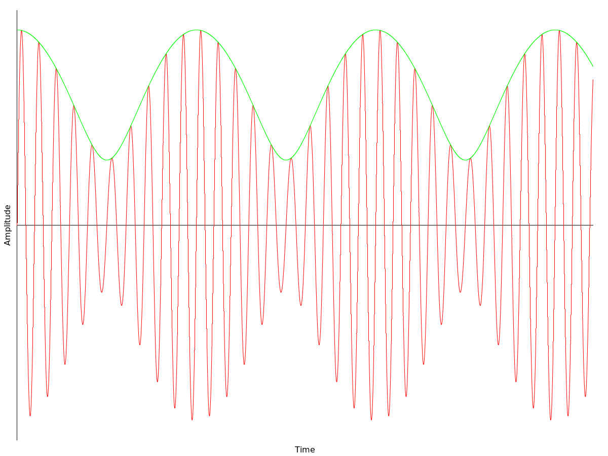
Let us now move on to the circuit in oscillating mode. As expected, injection pulling and injection locking of the oscillator occurs as the frequency of the input signal approaches the resonant frequency of the main tank. The transition from the occurrence of a distorted beat whistle to serious pulling of the oscillator's frequency towards the frequency of the input signal to the oscillator eventually being synchronized be the input signal is shown in the diagram below (the plot shows the envelope of the oscillations, details can be found in the full article).

What happens upon injection locking is that the carrier of the incoming signal is replaced by the local oscillations of the circuit, resulting in a carrier-boost effect. This carrier-boost is ultimately responsible for an increased selectivity of the receiver due to the properties of a typical envelope detector. An excellent introduction (in German) into this topic can be found here.
It should be noted that an oscillating regenerative receiver is fundamentally different from a true multiplicative homodyne receiver. In the latter, the input RF signal including it's original carrier is fed into a multiplicative mixer along with the locally recreated carrier to perform a frequency conversion directly into the audio frequency range. Again, an excellent introduction (in German) into this topic can be found here. However, with the oscillating regenerative receiver the carrier is simply replaced by a
local oscillation of much larger amplitude.
Finally, we can see that the "amplitude compression" effect and the resulting bandwidth widening is even more pronounced in oscillating mode. This is simply because the amplitude of the oscillations is much larger than the amplitude of the original carrier they have replaced. In the following diagram, an audio frequency curve for the receiver in oscillating mode is shown. Again, the reader is referred to the full article for details.

Obviously, the most striking feature of the regenerative receiver in oscillating mode is that in conjunction with the envelope detector it can achieve a high selectivity by virtue of boosting the carrier while at the same time even increasing audio frequency bandwidth.
The full article can be found here:
Attachments:
To thank the Author because you find the post helpful or well done.
SSB demodulation in oscillating mode
One one the most striking features of the oscillating regenerative receiver is the ability to demodulate single sideband (SSB) transmissions using it's envelope detector. The quick explanation for this behavior is that the local oscillations substitute the missing carrier of the SSB signal thus re-creating an AM signal suitable for the envelope detector in the receiver. However, like most quick explanations, this one has it's shortcomings, too. For instance: We only added the missing carrier to the SSB signal, in order to turn it into a regular AM signal one would have to add the missing other sideband as well. Why is adding only the carrier sufficient? Also, there is no carrier to injection-lock the local oscillations, how do we get the phase angle of the local oscillations right? (This is a trick question, we'll see later that we don't need to get the phase angle locked to zero in case of SSB.)
So let's take a more thorough look at the SSB demodulation process in the oscillating regenerative
receiver. First, we need a mathematical expression for a SSB signal. We'll choose upper sideband (USB), the considerations for lower sideband (LSB) are similar.

sUSB(t) then undergoes amplification in the transmitter, is broadcast and picked up by our antenna and appears with a certain amplitude "b" and phase angle "gamma" in the main tank of our receiver where it is added to the local oscillations with amplitude "a", creating an overall signal of

Fortunately, any phase shift between the local oscillations and the SSB signal can be added to the unknown phase angle "gamma" which manifests itself only in inaudible phase shifts in the AF signal. Hence, the local oscillations only need to have the correct frequency while phase locking is not necessary.
However, the envelope function h(t) of the beat is not quite the original AF signal contained in the transmission. In fact, the square root causes a severe distortion that is most pronounced when the amplitudes of the local oscillations and the SSB signal are equal as can be seen from the following plot (note the the time axis is not to scale):

Obviously, adding only the carrier and not the other sideband does not produce an exact AM version of the SSB signal, it merely leads to a more or less distorted version. The distortion is mitigated as the amplitude of the local oscillations becomes larger than the amplitude of the SSB signal. The following plot shows the beat envelope for the local oscillations having twice the amplitude of the SSB signal.
Hence, in order to produce a not overly distorted version of the original AF signal in the envelope detector we need to make sure that the amplitude of the local oscillations is considerably larger than the amplitude of the SSB signal. Mathematically, this can be seen the following way:

which is an envelope function as if the AF signal had been used in a regular AM transmission with modulation depth m=b/a and is therefore perfectly suitable for the envelope detector in our regenerative receiver.
To thank the Author because you find the post helpful or well done.
Overcoming The Grid Leak Detection Threshold
It has been mentioned in the paper on the oscillating regenerative receiver that the carrier boost effect that occurs when the circuit goes into it's oscillating state will improve envelope detection of the AF signal if the detector is non-linear and delivers a higher AF output voltage at higher RF input ampli- tudes. While in the paper the anode bend detector has been cited as an example, this also applies to the more frequently used grid leak detector. In fact, the carrier boost effect occurring in the circuit's oscillating state can be used to push the amplitude of small RF signals in the input tank well above the detection threshold of the grid leak detector.
Let's take a closer look at this. First, we need an understanding of how the detection threshold in a practical grid leak detector comes into existence. We shall start by looking at the grid voltage vs. grid current of a typical directly heated triode, the KC1, which has been used extensively in European battery powered regenerative receivers.

The dashed line in the above diagram shows an idealized I-V curve of a diode that has a sharp knee at a certain forward threshold voltage (400mV in the above example). In contrast, the grid leak current of our practical directly heated triode has a much wider knee stretching from approximately 250mV to 550mV.
For envelope detection to occur, the RF voltage URF(t) at the grid as a function of time obviously needs to include the knee in the I-V curve. Hence, the grid bias of the directly heated triode in our example should be chosen to be around 400mV. This is usually done by connecting the grid resistor to a voltage divider between the positive heater voltage (+2V in case of the KC1) and ground. While in case of the idealized I-V curve an arbitrarily small RF grid voltage centered around the bias of 400mV will fully include the sharp knee, this will not happen for practical grid leak I-V curves. Here, a small RF grid voltage (e.g. 100mVpp) will only include a part of the knee and hence yield only a small detected AF voltage.
Another way to look at this is the following: If the detection device behaved perfectly linear (like a resistor) no detection would occur at all. Hence, the more linear the detection device behaves within the input voltage range, the smaller the detected AF output voltage will be. If we look again at the above diagram, it becomes clear that for input voltages in the range of 100mVpp and smaller a linear approximation of the I-V curve would be quite accurate and therefore we expect only a small detected AF voltage for such small RF amplitudes.
Let's now measure the detection behavior of the KC1 grid leak detector for different RF amplitudes. This will be done using the setup depicted below:

The plate load resistor RA is 470kΩ, the supply voltage is U0=95V, the grid resistor Rg is 1MΩ and the
grid capacitor is 100pF. The grid bias is set to +400mV by the 1kΩ poti between the positive heater voltage (+2V) and ground. A low output impedance RF signal generator provides a variable amplitude RF input signal. The grid voltage Ug(t) including it's DC component is measured.
The way grid leak detection works, the average grid voltage varies with the amplitude of the RF signal and the detected AF content of the RF signal is in the average grid voltage varying at audio frequency. Therefore, a "detection diagram" for a specific grid leak circuit is a plot of the average grid voltage versus the amplitude of the (constant amplitude) RF signal. Such a detection diagram for the setup given above is shown in the following picture:

Using such a detection diagram to determine the detected amplitude of a sinusoidal AF signal from the RF signal's median amplitude and modulation depth is quite simple. First, the RF signal amplitude range given by the median RF amplitude and modulation depth is determined. The intersection of the lowest and highest amplitude of the RF signal with the detection curve then yield the maximum, resp. minimum average grid voltage on the vertical axis and hence the peak-to-peak AF signal amplitude. The detection threshold now becomes apparent: In order to produce a reasonable AF amplitude, the RF signal amplitude needs to be higher then approximately 200mVpp.
Let us now look at an RF signal with a median amplitude of 100mVpp and a modulation depth of 50%. The RF amplitude range is hence 50mVpp to 150mVpp. Obviously this hits the flat portion of the detection curve for small RF amplitudes and the resulting AF amplitude is maybe 2 or 3mVpp. If we now put the receiver in oscillating mode, injection locked to the incoming RF signal, the median RF amplitude increases drastically at the expense of the modulation depth. It has been shown in the paper on the oscillating regenerative receiver that boosting the carrier by a factor of µ will decrease the modulation depth by the same factor. Let's say we boost the carrier of our 100mVpp RF signal 10-fold to 1000mVpp, the modulation depth will simultaneously drop to 5%. This will lead to an RF amplitude range of now 950mVpp to 1050mVpp. From the detection curve, we can see that this will now yield a detected AF amplitude of approximately 30mVpp which is a large increase over the originally detected AF amplitude!
We are now able to give a conclusive answer as to why the regenerative receiver often appears to have a higher sensitivity towards small RF signals when put into oscillating mode. The underlying "mechanism" is indeed very simple: By putting the receiver into oscillating and injection locked mode, the resulting carrier boost will push small RF signals well over the detection threshold of the grid leak (or anode bend) envelope detector.
To thank the Author because you find the post helpful or well done.
High Feedback Oscillators
The work done so far on the oscillating regenerative receiver can, of course, also be applied to LC oscillators. In fact, single tank regenerative receivers and LC oscillators are often based on the same circuits. We shall now take a closer look at a very interesting case: The high feedback oscillator with real-time limited feedback. We shall use the inductive feedback circuit that was developed in post #1 of this thread. However, since we are looking at the circuit as an oscillator, the driving voltage Ud from the antenna is no longer present and we end up with the following circuit:

The reader is referred to the paper "Regenerative Circuits With Real-Time Feedback Limiting" from post #1 for a detailed description of the circuit. The feedback current If impressed by the controlled current source into the feedback coil is again modeled by
where UC is the voltage at the capacitor. Again, the reader is referred to the paper attached to post #1 for further details. To achieve a high feedback into the LC tank, we set b1=3mA and b2=10V-1 resulting in a very high small signal transconductance of 30mA/V. The following diagram shows the feedback current If as a function of the voltage UC at the capacitor.

Obviously, the feedback device reaches saturation very quickly. The other circuit parameters are as follows: The capacitance is C=100pF and L is chosen such that the resonant frequency of the tank is 1MHz. The shared inductance
is set to 2μH and the physical loss resistance R shall be 30Ω, resulting in a physical Q-factor of ap- proximately Q=53.
The positive feedback delivered into the LC tank replaces the physical loss resistance R with the (time dependent) virtual loss resistance
that, unlike the physical loss resistance, can be zero or even negative. A negative virtual loss resis- tance indicates that the feedback device is pumping more energy back into the LC tank than dissi- pated in the physical loss resistance. The reader is once more referred to the paper attached to post #1 and the references therein for an in-depth introduction of the concept of a virtual loss resistance and the derivation of the above equation.
Let us now look at the capacitor voltage and the virtual loss resistance as functions of time after the oscillator has reached stable operation (t0 is approx. 200μs).

Obviously, in case of very high transconductance, the feedback device is inactive for most of the cycle (this is simply because it reaches saturation very quickly) and the virtual loss resistance is equal to the physical loss resistance of 30Ω most of the time. The feedback device becomes active only twice in each cycle when UC is around zero and almost instantaneously replaces the energy dissipated in the physical loss resistance over the preceding semi-cycle. This almost instantaneous energy replacement twice in a cycle can nicely be seen by looking at the current I(t) in the LC tank along with the virtual loss resistance:

Each time the feedback device leaves the saturation region and becomes active around UC=0 the absolute value of the current I(t) in the tank gets "bumped up" to the value it started with at the beginning of the semi-cycle. Without these bumps, we would see an exponentially decaying amplitude of I(t). The following plot shows I(t) with these bumps enlarged.

It is noteworthy that the behavior of oscillators with real-time feedback limiting in case of high feed- back that has been seen here is fundamentally different from the high feedback behavior of oscillators with implicit automatic gain control (e.g. a tuned grid oscillator). The latter usually suffer from stability issues often leading to intermittent oscillations when the positive feedback is to high.
To thank the Author because you find the post helpful or well done.