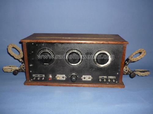
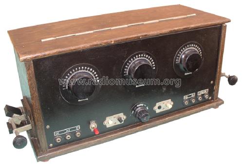
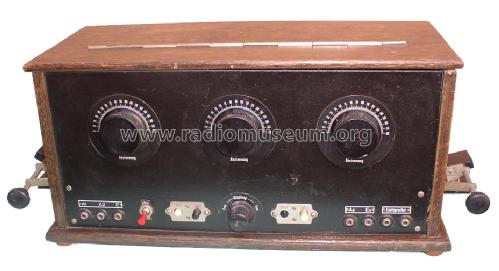
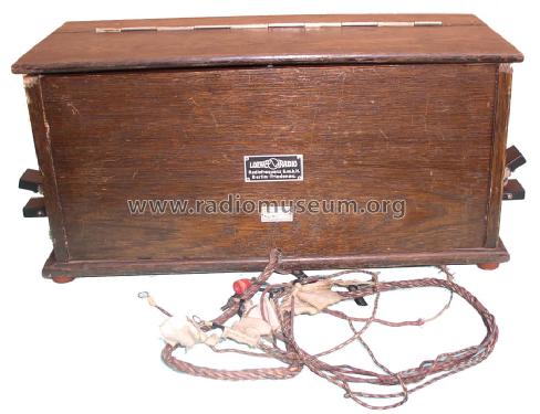
Fernempfänger 2H3N (2HF3NF) Batterie Steglitz
Loewe-(Opta); Deutschland
- Country
- Germany
- Manufacturer / Brand
- Loewe-(Opta); Deutschland
- Year
- 1927–1930
- Category
- Broadcast Receiver - or past WW2 Tuner
- Radiomuseum.org ID
- 2548
-
- alternative name: Löwe Radio
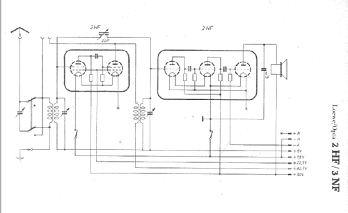

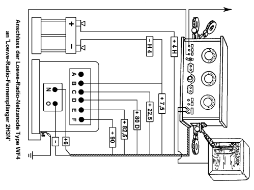
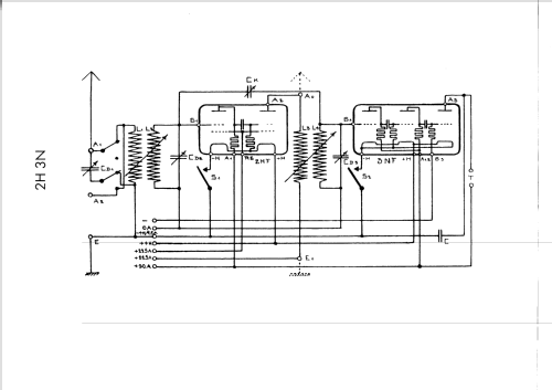

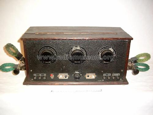
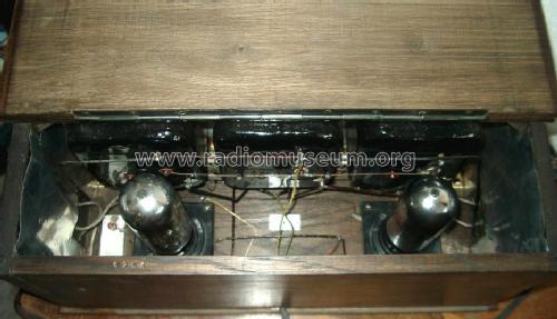
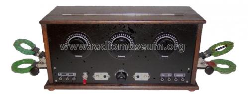
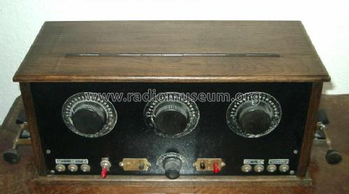
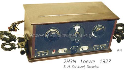
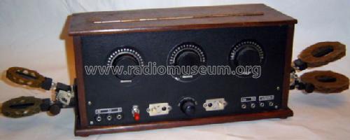
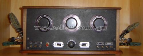
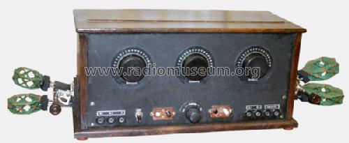
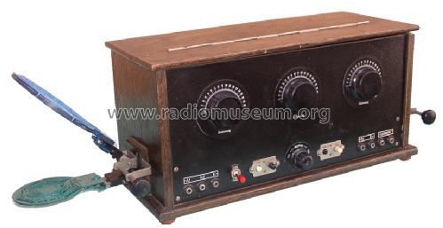
Mit Huth Spulenkoppler ab Werk
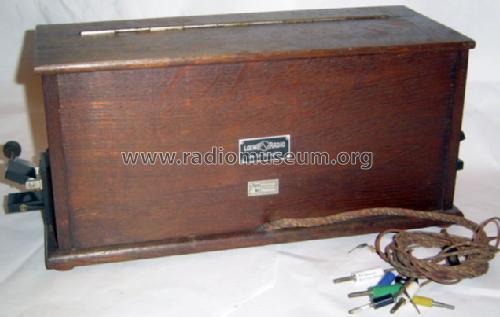
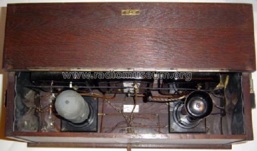
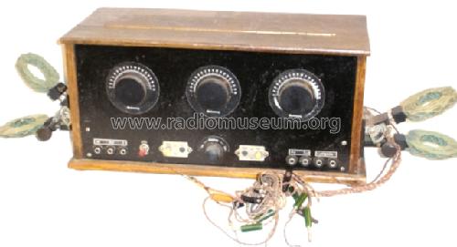
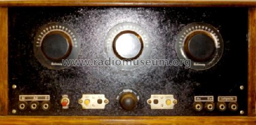
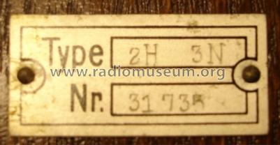
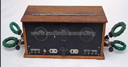
D Löwe 1927 2H3N
RKK Radio Museum --- www.rkk-museum.ru
RKK Radio Museum --- www.rkk-museum.ru

RKK Radio Museum --- www.rkk-museum.ru

RKK Radio Museum --- www.rkk-museum.ru

RKK Radio Museum --- www.rkk-museum.ru
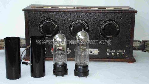
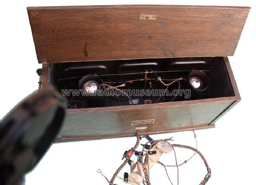
Mit den häufig fehlenden Röhrenabschirmungen
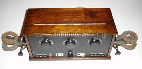
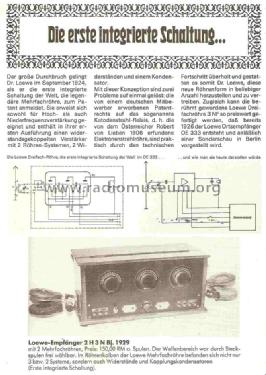
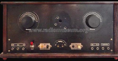
by courtesy of Maik Slotosch-Kemper
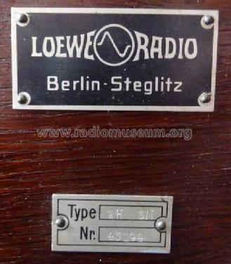
by courtesy of Maik Slotosch-Kemper
Click on the schematic thumbnail to request the schematic as a free document.
- Number of Tubes
- 2
- Main principle
- TRF with regeneration; 2 Special; 2 AF stage(s)
- Tuned circuits
- 2 AM circuit(s)
- Wave bands
- Broadcast (MW) and Long Wave.
- Power type and voltage
- Storage and/or dry batteries / 90 & 82,5 & 22,5 & 6 & 4 Volt
- Loudspeaker
- - This model requires external speaker(s).
- Material
- Wooden case
- from Radiomuseum.org
- Model: Fernempfänger 2H3N Batterie [Steglitz] - Loewe-Opta; Deutschland
- Shape
- Tablemodel, Box - most often with Lid (NOT slant panel).
- Dimensions (WHD)
- 430 x 210 x 185 mm / 16.9 x 8.3 x 7.3 inch
- Notes
-
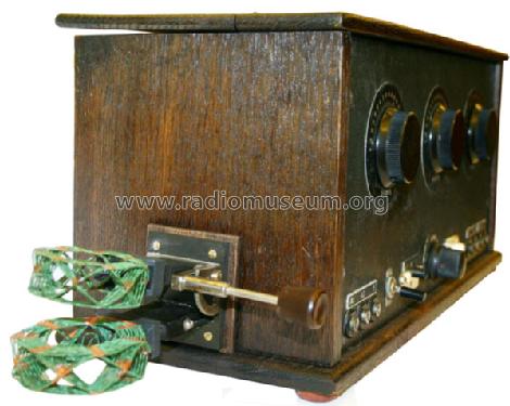
Steckspulen-Koppler an beiden Seiten; 200-4000 m.
[306,509,512,514,559,560] Das Gerät gab es in einer älteren Ausführung mit dem Herstellerschild "Loewe-Radio Berlin- Friedenau" und nach dem Umzug der Firma 1927 mit "Loewe-Radio Berlin- Steglitz"
- Net weight (2.2 lb = 1 kg)
- 5.4 kg / 11 lb 14.3 oz (11.894 lb)
- Price in first year of sale
- 145.00 RM !
- Source of data
- Katalog Radio-Zentrale Prohaska 1928 / Radiokatalog Band 1, Ernst Erb
- Circuit diagram reference
- Lange-Nowisch
- Mentioned in
- Funkgeschichte der GFGF (8969)
- Literature/Schematics (3)
- Le Guide du Collectionneur TSF Biraud/Foster, Vol. I (page 223)
- Picture reference
- Das Modell ist im «Radiokatalog» (Erb) abgebildet.
- Other Models
-
Here you find 1646 models, 1383 with images and 1189 with schematics for wireless sets etc. In French: TSF for Télégraphie sans fil.
All listed radios etc. from Loewe-(Opta); Deutschland
Collections
The model Fernempfänger is part of the collections of the following members.
- Konrad Birkner † 12.08.2014 (D)
- Klaus Dräger (CH)
- Thorsten Finaske (D)
- Wolfgang Flügel (D)
- Markus Glaser (D)
- Valery Gromov (RUS)
- Axel Harten (D)
- Gregor Hoebrink (D)
- Nico Jacobsen (D)
- Wolfgang Kobler † 21.11.18 (D)
- Zlatan Mumlek (HR)
- Thomas Neumüller (A)
- Timo Rantasaari (FIN)
- Karlheinz Schneider † 28.6.23 (D)
- Hans Stellmacher (D)
- Jürgen Stichling (D)
- Albert Vonarburg (CH)
- Hartmut Völler (D)
- Eckhard Wegner (D)
Museums
The model Fernempfänger can be seen in the following museums.
Forum contributions about this model: Loewe-Opta;: Fernempfänger 2H3N Batterie
Threads: 4 | Posts: 4

Fellow Radiophiles,
For the writing of this post, I am deeply indebted to RM member and author of the book "Die Loewe Mehrfachröhren" - The Loewe Multi-Tubes, Gerhard Eisenbarth.
I dedicate this post to Ernst Erb, the founder of our host organization Radio Museum Foundation of Lucern [18], on his 90th birthday May 20th and to many long time collaborators and good friends, including Eng. Hans Knoll and the late Prof. Dr. Dietmar Rudolph.
This post is divided into 50 sections to help navigate and to make it easy to go directly to a topic of interest. The 50 sections are listed in the Table of Contents after the introductory text. There is a return link to the table of contents at the end of each section. When you jump to a section, you can go back to the jumping point with the back-key in your browser.
All pictures and diagrams can be clicked to expand in a separate window.
2026 marks the 100th anniversary of the launch in Germany of the Loewe 2H3N Fernempfänger (Long distance, DX radio) with two multi-tubes and the simpler version, the Loewe OE333, with one multi-tube for local station reception.
An internal Loewe document states the following about the market launch [1, p 1.40]:
"August 16, 1926: The Loewe OE333 local receiver with the 3NF triple tube is presented as a major innovation at a special radio show in Berlin, Leipzigerstrasse, where it goes on sale at the sensational price of RM 39.50 (without plug-in coils). Demand for this popular device for loudspeaker reception soon became so high that daily production had to be gradually increased to 2,000 units."
"September 3, 1926: At the 3rd Radio Exhibition, the OE333 local receiver and the 2H3N long distance receiver, each with a double and a triple tube, are presented. The 2H3N receiver was later also manufactured in large quantities and exported to many countries."
The market launch of the OE333 at the end of 1926 triggered a surge of competition in the radio industry. Until then, a radio with three tube stages cost well over RM 100. The Loewe local receiver, priced at RM 39.50, also triggered a sales boom because it met the interests of the growing radio audience for inexpensive devices. Due to the widespread economic hardship among large sections of the population at the time, the Loewe device came at just the right moment. Many people could now afford a radio at this price [1, p 1.46].
I acquired the Loewe 2H3N Fernempfänger recently from an American collector through an on-line auction for $497USD.
The multi-tubes (double and triple tubes) are glass envelopes with several RC-coupled triodes in hard vacuum. Some multi-tubes also feature tetrodes and pentodes. I will refer to these tubes with multiple triodes inside as multi-tubes to avoid confusion with "tube" representing one triode, or representing the whole assembly with several triodes.
The original set of multi-tubes from 1926 had thoriated tungsten filaments. The two tubes were the 2HF dual space charge tetrode RF amplifier and the 3NF detector, preamp and power amp with three internally RC-coupled triodes.
My set came equipped with the later generation of multi-tubes with higher emission Barium coated cathodes: the HF30 with 2 triodes wired as an RC-coupled RF amplifier and the 3NFB with 3 triodes including anode bend detector, audio preamp and audio power amp. The resistors and capacitors were developed and manufactured by Loewe and sit in their own sealed glass envelopes to avoid contaminating the hard vacuum for the triodes. All triodes in the HF30 and 3NFB operate in common cathode configuration, with the filaments wired in series. The original 3NF had the two input triode thoriated filaments in series and the filament of the power triode in parallel with the other two.
This acquisition gave me the opportunity to measure the properties of the two multi-tubes (Mehrfachröhren HF30 and 3NFB), to evaluate the radio's performance and how the radio made use of the two Loewe integrated multi-tubes. I also created simulation models from measurements of the HF30 and 3NFB to explore the operation of the 2H3N further in LTspice simulations, including probing the internal operation of the multi-tubes in ways that are inaccessible in practice. I also compare measured radio performance with simulated results to be sure that the models and simulation are correct.
Shortly after I acquired this radio, I also obtained a copy of the fantastic German language book "Die Loewe Mehrfachröhren" [1] by RadioMusuem member Gerhard Einsenbarth (his forum posts). Gerhard is a retired engineer and specialized in the development of color display CRTs (Cathode Ray Tubes). His professional knowledge was invaluable to ensure rigor and to deepen the technical content of the book. I read the book cover-to-cover. The author gives a comprehensive history of the technology and business of the production of these tubes with many references. The book is in large format with 370 heavy stock pages on which some 800 high quality photos and diagrams are included. Many of these include detailed photos of the interior components of the multi-tubes. This book also reads like an extraordinary adventure. I count this book as one of the great dividends of learning the German language starting circa 2009, to be able to read the excellent German text content at RadioMuseum. The book only exists currently in print form and is in short supply. An English language translation in eBook form is being created. The publisher is the GFGF (Gesellschaft der Freunden der Geschichte des Funkwesens - The Association of the Friends of the History of Broadcast Science). This is the German language antique radio club. You can find it on the web at GFGF dot ORG.
This book served as the central reference for my analysis of the radio and its multi-tubes, and for this article. As I read the book and worked on the radio, I was in frequent correspondence with its author Gerhard in German, but the author can also correspond in English.
Die Loewe Röhre 3NFB - Analyse einer Mehrfachröhre is a small section of the book about the specifics of the 3NFB low frequency multi-tube. Use a German language translator if needed. You can get a Google translated version of any post in the forum by hitting the flag icon at the top of each post. The author has updated his calculation of the 3NFB parameters in the more recent "Die Mehrfachröhren". I used his updated calculation.
The Loewe line of multi-tubes started a revolution in the German radio market. No other company ever integrated resistors and capacitors inside the tube envelope. It is fair to say that there were almost no resistors available as components, aside from wire-wound types, or high-MegΩ grid-leak resistors. The multi-purpose resistor component had not been invented yet. Loewe launched a range of its vacuum encapsulated resistors and capacitors with the development of the multi-tubes. The most important technical consequence for the integrated approach was the higher performance in terms of gain and bandwidth as well as reduced outside interference pickup. Additionally, each triode was carefully optimized for its specific function in each multi-tube. The invention of this integrated component concept came from company founder Sigmund Loewe, who also enlisted the help of Manfred von Ardenne for a few years to help optimize the design of the tubes and to participate in other development work. S. Loewe had two other brothers involved in the business: David Loewe and Bernhard Loewe. For more historical details about Loewe, please check the Loewe company profile page.
From the point of view of an American collector, the multi-tubes represent an extraordinary leap in performance. From 1920 until about 1927, nearly all American radios were made with the 00, 01, 01A triodes. These were marked with additional prefix letters and numbers to designate the base type, licensed manufacturer and other construction details (i. e. UV01, UV201, CX300, etc). This class of triodes was originally developed for reliable telephone repeater service in long distance lines (search for "The Vacuum Tube Saga" by Gerald Tyne. It is hosted by MIT). The large V-shaped filament cathode sat inside a large rectangular box-shaped grid. These sat in a box shaped plate. This worked reliably for audio, but was terrible for RF performance due to the extremely high internal capacitance of 8pF from grid to anode (Cga). The Cga=8pF made the tubes very prone to oscillation in RF amplifier circuits in a radio. A filamentary RF triode with a cylindrical plate would have Cga=2-3pF.
The form of the triodes in the Loewe multi-tubes is the classic cylindrical form, with cylindrical anode, spiral grid with a single filamentary cathode wire along the axis of the cylindrical form. Similar to the TM model from 1915. This simple form made it possible to optimize the triode design for RF use with low internal capacitance. I measured 2.8pF from anode to cathode (Cga) in the HF30 2-stage RF amplifier. The cylindrical triodes were also optimized for very high voltage gain of mu=57 for service as anode bend detector and as audio preamp in the 3NFB. By comparison, the American 01 tube was limited to a voltage gain of mu=7. For most of the 1920's, RCA had the US monopoly on the manufacture of conventional triodes. Aside from the obvious existence of the RCA monopoly, it is still a mystery how the misfit 01 triode was chosen by RCA in the mid 1920s as the tube for all radio design, including RF and audio, by countless manufacturers in the American radio industry, including RCA's own radio designs.
A German language version of this post is also planned for our German speaking fellow radiophiles.
Linked Table of Contents
-
Operating the OE333 Configuration with a Large Indoor loop Antenna
-
Comparing Anode-Bend to Grid-Leak and 1N34 detector in the OE333
-
The 2HF Space Charge Tetrode Multi-Tube in the First Version 2H3N
1. Architecture of the Loewe 2H3N
The model name 2H3N is an abbreviation for 2 Hochfrequenzröhren (2 high frequency valves) in the HF30 and 3 Niederfrequenzröhren (3 low frequency valves) in the 3NFB. Two variable coupling air coil transformers couple into and out of the RF amplifier HF30. The second RF transformer couples directly into the 3NFB anode bend detector, followed by one stage of preamplification. The third triode in the 3NFB drives a high impedance speaker directly.
Click the figure to enlarge

The tube filament power comes from a 2-cell 4.2V lead-acid battery with the negative terminal tied to ground. I verified that the 250mA filament current from both tubes causes a voltage drop across the filament power wires, H+ and H-, of about 0.2V. This reduces the nominal 4.2V at the battery to close to 4V at the filaments of the HF30 and the 3NFB. Unlike with contemporary American radios that had 5V filament tubes running from a 6.3V battery, which required a voltage regulating rheostat in series, the multi-tubes were designed to operate directly from the 4.2V battery.
All DC bias and supply voltages come from taps in the 90V HV battery pack (Anodenbatterie), as was common with contemporary radios. The HV pack supplies the anode voltages, 90V and 82.5V. The 7.5V tap is tied to ground, so that the 6V tap provides -1.5V grid bias to the input grids of each multi-tube and the 0V HV battery tap provides a -7.5V bias source for the output audio power triode.
There are no fixed resistors outside the integrated multi-tubes and there are no rheostats. The only other component that is external to the tubes is the 5nF filter capacitor between the audio output anode that drives the high impedance 4kΩ speaker and ground. The volume is controlled by adjusting the angle of the variable coupling RF transformers.
Keep in mind that the carbon composition resistor had not been invented yet in the mid 1920's. So the multi-tubes pioneered the first wide range high quality precision thin film carbon resistors. Essentially all sets up to 1926 were operated from batteries and may have had only one high value carbon film resistor as part of the grid leak detector, which value ranged in the 1MΩ to 10MΩ and maybe only 50% accuracy. The other resistors in competing early sets were all wire-wound rheostats from a few ohms up to a few kΩ. Wirewound resistors are also useless for RF work due to their high inductance and capacitance parasitics. The glass encapsulated resistors and capacitors from Loewe were also sold individually as very high quality resistors. See Loewe discrete resistors and capacitors and Loewe resistors. Some of the resistors show a spiral cut through the resistive film, as you might find in modern thin metal film resistors.
Two tuned RF transformers with variable coupling. The radio has four plug-in coils. The first, second and fourth coils are tuned LC tanks with three fully shielded variable capacitors. The third coil serves as the high inductance primary with variable coupling the the third and last tuned LC tank.
 The KURZ/LANG switch at the input tank. This switch connects the external antenna to the input LC tank in series with KURZ (short) or in shunt with LANG (long). The antenna could be a long wire, a short wire or a large loop antenna. However, the original intended application of these two switch settings was not specified in the operating instructions. Just going from the meaning of the two words, one might think that LANG is for long antennas, like >50m (~150ft), which have a relatively large equivalent capacitance (450pF, -j350Ω reactance at 1MHz, 300m wavelength) as an electrically short antenna as compared to 300m at 1MHz. But the LANG selection places the 30pF-560pF tuning capacitor in parallel with the antenna coil L2 and antenna, thus greatly liming the tuning range, where the total capacitance can only vary from about 450pF+30pF=480pF to 450pF+560pF=1010pF. This limited tuning range in LANG also lowers the resonant frequency and increases the resonant wavelength, thus tuning longer wavelengths. Switching to the KURZ position connects the input coil, the tuning capacitor and antenna capacitance all in series. Now the input LC tank configuration makes much more sense with a much wider tuning range with the variable capacitance ranging from a few 30pF to 1(1/450pF+1/560pF)=250pF. With this smaller maximum capacitance it becomes possible to tune higher frequencies and shorter wavelengths in KURZ (short) position. So, LANG for longer waves and KURZ for shorter waves; this only applies for long 30m to 50m antennas with high self-capacitance. But this is only my interpretation of the circuit.
557pF Tuning Capacitors: The three tuning capacitors have a relatively high maximum specified value of 557pF (500cm*1.113 pF/cm). The cm unit in the set data is an obsolete CGS unit of capacitance, where 1.113pF=1cm*1.113pF/cm. All three capacitors have grounded full metal shields. One effect of the relatively high tuning capacitance, which is about twice the typical 250-350pF tuning capacitor found in other contemporary radios, is to lower the impedance of the tank to better drive the slightly reduced input grid impedance of the HF30. The input 30pF-560pF tuning capacitor was measured in the set with the HF30 input grid connected to it and the power turned off.
Conversely, with a very short antenna, like 5m, the equivalent antenna capacitance is much smaller (53pF) and the impedance much higher (-j3000Ω at 1MHz). In this case, the LANG position loads the antenna with the input LC tank wired in parallel with tuning range from 30pF+53pF=83pF to 53pF+560pF=610pF. In series, the capacitance range would be from 1/(1/30pF+1/53pF)=19pF to 1/(1/560pF+1/53pF)=48pF. So, the Lang position is useful for short wire antennas.
2. Plug-in coils
My set came with the set of coils shown in the photos. Loewe also marketed a full set of coils for the 2H3N to cover reception in the LW and MW bands.

I also already had a few recently made coils and attached some of them to banana plugs that go directly into the sockets in the 2H3N. The spacing of the coil pins is the same as in a modern 220VAC European power plug. They also fit most lab voltmeter banana sockets. These coils were made in 2009 by John Bruckner. See the earlier report about "Beautiful Coils". I own two of the green solid wire coils below, which I usually use for L2 and L4 during radio operation. The solid wire green coil in the center and the Litz wire coil on the right have a tap switch that taps into about half the turns. The active part of the coil is the outer part, while the inner part remains connected at the tap with the other end left open.
You may have seen, that in schematics with tapped coils, the tapping is often done by shorting a few turns to reduce the total inductance. This is often done for LW vs MW band selection. The advantage of the shorted method is that the unused part of the coil is not allowed to resonate at its self resonant frequency. I have found that the unused part of the two coils on the right, which is open, tends to self-resonate around 2MHz. But shorting half the turns would reduce the total inductance further than leaving them open because the unused portion of the coil is too tightly coupled to the active part of the coil. In order to get the same inductance with an open unused coil section as a shorted unused coil section, I would have to short fewer turns.

I have experimented with all the coils you see here, so I decided to measure the inductance and Q at several frequencies with the frequency sweep method while the coil is tuned to the desired frequency.
The inductance L was measured with the Rhode&Schwarz LRT BN 6100. This instrument resonates the coil under test with an internal 5nF capacitor and you sweep the frequency manually with the dial knob to achieve a peak reading in the analog meter. The 5nF forces the resonance below the typical application frequency and is thus very insensitive to stray capacitance. Even the coils in IF transformers with internal capacitors can be measured without disconnecting the fixed resonant capacitor, because the internal capacitor is likely under 100pF. The BN6100 also offers a measurement to find the self-resonant frequency with the internal 5nF capacitor disconnected. This would give the approximate value of the internal capacitor in the IF transformer. This is a reliable instrument, but I have not gotten good results measuring Q. This Q measurement, even if accurate, is not useful because it is done at much lower frequencies than the coil will be operated in.
The new coils by John Bruckner have a much lower Q than his published result as measured with his "Calibrated TS-617C/U Q-meter". John gets results in the high 100's. My top Q for the new coils is only 232 for the single layer Litz wire coil at 413kHz. The resonance method is usually fool proof. Maybe I have unaccounted losses in the wiring or in the capacitor itself. My Q measurements are useful in this context, because it is the Q that is achievable in the radio. The frequency at which the Q is measured is very important, as the coil Q varies a lot with frequency, as much as by 2 to 1.
The best method to measure coil Q is to sweep the frequency with the coil resonated with a tuning capacitor to the frequency of interest for the Q as follows:
The Q is measured from the bandwidth at resonance as Q=Fpeak/Fbandwidth.
The capacitance is measured from the peak frequency Fpeak and inductance as C=1/(L*4*π2*F2)
The reactance XL is calculated from the inductance as XL=L*2*π*Fpeak.
The tank equivalent shunt resistance resistance at resonance is measured from Q and the reactance as Rshunt=XL*Q. The equivalent series resistance is Rseries=XL/Q. In practice, the series and shunt equivalent resistance should be apportioned so that a reasonably accurate Q is achieved over the entire AM band from 500kHZ to 1500kHz. Series resistance lowers the low frequency Q and shunt resistance lowers the high frequency Q.
The following is a summary of my measurements of all the coils at various frequencies of interest, from 362kHz to 1997kHz. The table is sorted on the first column by decreasing inductance. The Q and equivalent shunt resistance at the resonant frequency Fpeak will be useful to see the coil loading effects in the 2H3N radio, that are caused by the input and output of the HF30 and input of the 3NFB.
| L (uH) | Fpeak (kHz) | Q | C (pF) | XL (Ω) | Fpeak Res (kΩ) | Coil type |
| 2600 | 362 | 42 | 74.3 | 5914 | 248 | Old large waffle |
| 410 | 501 | 38 | 246.1 | 1291 | 49 | Old small tight |
| 410 | 909 | 28 | 74.8 | 2342 | 66 | Old small tight |
| 410 | 914 | 31 | 74.0 | 2355 | 73 | Old small tight |
| 250 | 413 | 232 | 594.0 | 649 | 151 | New Litz wire flat waffle |
| 250 | 414 | 197 | 591.2 | 650 | 128 | New Litz wire flat waffle |
| 250 | 500 | 192 | 405.3 | 785 | 151 | New Litz wire flat waffle |
| 250 | 500 | 207 | 405.3 | 785 | 163 | New Litz wire flat waffle |
| 250 | 1001 | 70 | 101.1 | 1572 | 110 | New Litz wire flat waffle |
| 250 | 1132 | 95 | 79.1 | 1778 | 169 | New Litz wire flat waffle |
| 241 | 500 | 85 | 420.4 | 757 | 64 | New solid wire waffle |
| 241 | 1001 | 54 | 104.9 | 1516 | 82 | New solid wire waffle |
| 241 | 1156 | 74 | 78.7 | 1750 | 130 | New solid wire waffle |
| 238 | 424 | 202 | 592.0 | 634 | 128 | New Litz wire layered waffle |
| 238 | 500 | 184 | 425.7 | 748 | 138 | New Litz wire layered waffle |
| 238 | 1000 | 69 | 106.4 | 1495 | 103 | New Litz wire layered waffle |
| 238 | 1146 | 49 | 81.0 | 1714 | 84 | New Litz wire layered waffle |
| 102 | 645 | 175 | 596.9 | 413 | 72 | New Litz wire flat waffle |
| 102 | 1000 | 119 | 248.3 | 641 | 76 | New Litz wire flat waffle |
| 102 | 1500 | 52 | 110.4 | 961 | 50 | New Litz wire flat waffle |
| 102 | 1702 | 32 | 85.7 | 1091 | 35 | New Litz wire flat waffle |
| 92 | 698 | 73 | 565.1 | 403 | 29 | New solid wire waffle |
| 92 | 1000 | 68 | 275.3 | 578 | 39 | New solid wire waffle |
| 92 | 1497 | 44 | 122.9 | 865 | 38 | New solid wire waffle |
| 91 | 706 | 78 | 558.5 | 404 | 31 | Old medium waffle |
| 91 | 706 | 78 | 558.5 | 404 | 31 | Old medium waffle |
| 91 | 1496 | 46 | 124.4 | 855 | 39 | Old medium waffle |
| 74 | 769 | 74 | 578.8 | 358 | 26 | Old small waffle |
| 74 | 1000 | 76 | 342.3 | 465 | 35 | Old small waffle |
| 74 | 1501 | 54 | 151.9 | 698 | 38 | Old small waffle |
| 74 | 1997 | 25 | 85.8 | 929 | 23 | Old small waffle |
You could copy and paste the contents of the table into your own spreadsheet, if you want to sort the table elements on any of the columns
The following are a few examples to illustrate the sweep results. Click plots to enlarge.


The frequency sweep signal is 10Vp-p and was generated to sweep the frequencies shown in the X axis of the plots with an HP3314A signal generator. I drove each tank with 1Meg or 3.3Meg source impedance to minimize tank loading. In the higher Q circuits, a significant amount of the signal drive to the tank was through stray capacitance. This is of no consequence to Q or bandwidth. The source impedance driving the tank just needs to be high enough and the stray capacitance simply becomes part of the calculated capacitance value.
The signal was collected with a 10Meg//20pF 10x probe into an HP54601B digital oscilloscope in "Peak Detect Display Mode". This mode detects the RF envelope by accumulating the +/- peak values. These are displayed in an alternating sequence that looks like a solid envelope with vector display mode turned on. A GPIB port in the scope ties to the USB-A port in the Windows 11 PC via a National Instruments GPIB-USB-HS adapter. See section "49. 48. Test Equipment Notes" below for more details. A Matlab script reads the envelope curve with alternating positive and negative values and takes their magnitude. Then a simple 10 point wide boxcar filter smooths the 1000 sample points to reduce noise. The 10 point box-car filter limits the horizontal frequency resolution to 1% of the sweep width. This is one reason why I narrowed the sweep to 20kHz around 500kHz for the highest Q=207 coil, L=250uH, shown in the center plot immediately above. The entry in the table for this coil showing Q=192 at 500kHz was done with a wider less precise 100kHz sweep. The other two plots cover 200kHz. The sweep duration of 100ms was adequate to eliminate curve distortions, provided the frequency sweep was short enough for the higher Q measurements.
I used the coil plug of the antenna circuit in the 2H3N as a handy test fixture and used the first tuning capacitor to tune the tank to the desired frequency. The KURZ/LANG switch was set to KURZ and a short banana cable jumper shorted A1 to E on the front panel.
Using the Plug-in coils in the set: The first tank resonates with the external antenna and is mounted on a variable 0-90o hinge to adjust coupling into the second stationary tuned tank, which is fixed horizontally under the first tank. The variable coupling optimizes signal coupling and selectivity into the RF amplifier in the HF30 multi-tube. Impedance matching between the antenna circuit with L1 and the second resonant tank with L2 by selecting coils with different numbers of turns. The variable coupling also serves to control overall gain, with the lowest coupling in the 90o position. Variable coupling is much more versatile for various signal conditions than RF stages with fixed coupling transformers that were standard in contemporary American TRF sets with 3 tuned tanks.
My favorite antenna at home is a large indoor 4-foot (1.2m) by 8-foot (2.4m) vertical loop made with CAT-5 Ethernet cable (see below in section 4. Four foot by Eight foot Loop Antenna). Unlike with long wire antennas that are shorter than 300m/4 (<<75m) at 1MHz, which have a lossy capacitive impedance, loop antennas have an inductive impedance with low losses. I use two pairs of Ethernet sockets to configure the 4 wire-pairs in the cable for 2 turns with 39uH and a self resonant frequency of 1360kHz or 4 turns with 165uH, but higher self-capacitance and a self resonance of 800kHz. Both of these self-resonant frequencies can be raised with a low value shunt inductance plug-in coil at L1 in the antenna tank, with the KURZ/LANG switch in the LANG (shunt) position.
I use the 2-turn 39uH loop most of the time, tuned in series (KURZ) with the 25-turn 74uH plug-in primary coil for frequencies below 1MHz and switched to shunt (LANG) to raise the tuning range for frequencies above 1MHz. Around 1MHz, either position works fine, but with different settings of the antenna tuning capacitor C1. Loop antennas collect signal from the magnetic RF field and are thus immune from the electric field interference noise that typically comes from electrical devices. Keep in mind, however, that loop antennas are directional, with a sharp notch in the direction of the axis of the loop. If you mount the large loop on a wall or back of a book case, select an orientation that receives the stations you are interested in. Even without any man-made electrical noise, the loop antenna still has an inherent 3dB SNR advantage because half of the received atmospheric static power is eliminated by the loop's receiving notch.
Keep in mind, that the Kurz/Lang (series/shunt) setting changes the tuning range of an inductive loop antenna in the opposite direction of an electrically short capacitive wire antenna. For example, a LANG (shunt) connection to a loop antenna raises the frequency of the tuning range of the antenna circuit, while it lowers the frequency of the tuning range of an electrically short capacitive wire antenna. In any case, this becomes obvious as you experiment.
 The second tank drives the input grid of the HF30 2-triode RC-coupled RF amplifier. It is biased with -1.5V to ground. This is the +6V tap on the HV battery pack, which is grounded at the +7.5V tap. Click the figure to enlarge.
There is no danger of oscillation with this connection because the first triode anode is loaded with an internal 33kΩ resistor, which is AC-coupled with an internal vacuum-sealed 85pF mica capacitor to the grid of the second triode. An inductive load on a triode would feed back to the grid through the Cga (grid-anode capacitance) and reflect as a negative conductance (inverse of impedance) at the triode grid. A negative conductance could then overcome the inherent positive conductance losses of the tuned tank at the grid and break into oscillations. The second triode grid is biased with the internal 33kΩ resistor tied externally to ground. The first triode filament is at ground level and the second triode filament sits in series between +2V and +4V from the lead-acid accumulator. The grounded bias resistor of the second triode gives a -2V bias with respect to the low end of its filamentary cathode.
3. The Coil Coupling Angle between High-Q Resonant LC Tanks
The coil coupling factor K is a strong function of the resonated Q of each coil and also of the distance and angle between the coils. The adjustable angle between L1-L2 pair and L3-L4 pair varies the coupling factor K. I refer you to this reference on Inductively Couple Circuits by Landee, Davis and Albrecht [15] for an extensive treatment on coil inductance, mutual inductance and coupling factor.
 I made measurements of the frequency response at the primary and secondary with excitation of the primary by a frequency sweep from 900kHz to 1100kHz. The 2H3N receiver was powered off. The coils were the identical modern pair shown above with green plastic insulation. I used their 91uH, 95uH taps for the tests. The case with identical coils is a special case and serves to illustrate ideal conditions with two high-Q resonated coils. Their Q is nominally 68 at 1MHz.
The intended use for the L1-L2 is with L1 connected to a long wire antenna, which has low Q and an impedance of a few hundred ohms in series with a few hundred picofarads. We will explore this case later.
 For these measurements and simulations, I am driving the L1 tank with the low loss step-down transformer coupling seen in the schematic on the left.
Both L1 and L2 are resonated by their respective capacitors C1 and C2. The blue curve shows the response at L1//C1 and the red curve shows the cumulative response of L1//C1 coupled into L2//C2.
The intended use for L3-L4 is with L3 not resonated at all, except for the self-resonance from its parasitic capacitance, while L4 is resonated with C3 in a narrow band high Q circuit. L3 is driven by the output anode of the HF30, which has an impedance in the 10kΩ to 25kΩ range. This will be measured and simulated later too.
The following eight measured frequency sweeps show the frequency response of the voltage at L1 and L2 as a function of coupling angle from 90o at right angles to each other to completely parallel with a 0o coupling angle. Keep in mind that even with 0o angle, there is still a 1.5cm (0.6inch) between the parallel coils. The input response at L1 is in blue and the output response at L2 is in orange. This gap limits the coupling factor K to 0.23, as shown in the last of the 8 sweep measurements below.
The peak values and bandwidth for both curves are reported near the top and bottom of the plots. The Q calculation that is shown is just the 1MHz center frequency divided by the bandwidth. These Q values are not the native Q of each resonant tank. The values reported as R1 and R2 are in kΩ and are the equivalent shunt resistance from the calculation if this Q-like value were the Q of a simple uncoupled LCR tank. The shunt resistance calculation is Rshunt=Q*XLC. The magnitude of the reactance is relatively low at 580Ω at 1MHz for all L and C.
Click to magnify
| 90o - K=0.0042 | 80o - K=0.0061 | 75o - K=0.0084 | 55o - K=0.015 |
 |
 |
 |
 |
| 45o - K=0.022 | 35o - K=0.0364 | 22o - K=0.059 | 0o - K=0.23 |
 |
 |
 |
 |
The measured frequency sweeps above show under-coupled response for 90o, 80o and 75o, critically-coupled response for 55o, where the input and the output levels are equal and the secondary reaches its highest signal level. For lower coupling angles from 45o down to 0o the response is over-coupled and develops a double peak, the output. It is almost amusing that the critically coupled response occurs about 45o. But the angle selection is a strong function of the Q of each coil. A higher Q would increase coupling, so that the maximum critical coupling that occurs currently at 55o would occur at a higher, more spaced out, angle.
 After the making the measurements, I simulated the coupling factor K empirically to get the same curve shapes as the measurements. The first curve is black and starts with the lowest value of K. The colors match between the three panels.
Panel 1 on the right shows the voltage at L1 as V(a2). The K factors are listed in the first simulated panel on their right. The curves are colored with the same sequence of K, starting with the black trace.
Panel 2 shows the voltage at L2. Note how the output at 1MHz peaks with critical coupling when K=0.015, which is obtained in the radio with a coupling angle of 55o between L1 and L2.
One comparison factor between measurement and simulation was the ratio of the signals at L1 vs L2 at 1MHz, which is shown in the 3rd panel on the right.
 I copied the simulated K factors to the angles in the measurement above, so that you have an idea of how much coupling there is between two identical high-Q coils, with Q=68.
The separate plot on the right is for the very over-coupled case with K=0.23, which, as with the measurement required a wider 800kHz-to-1200kHz sweep.
These measurements and simulations for high-Q coupled coils are useful when a high Q loop antenna is wired in series with L1.
You can find the corresponding simulatable schematics, symbols and plot command files section 50. LTspice Schematic, Symbol and Plot File Downloads. Rename the file extensions as directed.
4. Four foot by Eight foot Loop Antenna


The photos show the 4 foot-by-8 foot (1.2m-by-2.4m) antenna loop in my home lab. The loop is made of two turns of four conductors each, inside CAT5 Ethernet cable. The extra set of Ethernet sockets can reconfigure the loop into 4 turns of 2 wires for each turn.
| Inductance (uH) | Quality factor | Self Capacitance (pF) | Self Resonance (MHz) | |
| Loop2T | 39 | 65 @ 850kHz (900pF total) | 350 | 1.36 |
| Loop4T | 111 | 55 @ 450kHz (1140pF total) | 440 | 720 |
The Loop2T is best for the upper half of the MW band and if above 1.3MHz, you need to place the Kurz-Lang switch in the Lang position, that places L1 in parallel with the 39uH of the Loop2T to extend the tuning range. With L1=74uH from the old small waffle plugin coil the parallel inductance is reduced to 26uH and the self-resonance frequency is raised up to 1.68MHz.
5. Coupling between Low-Q and High-Q Resonant LC Tanks
Now we take a look at coupling between a low Q L1 circuit and a high Q L2 circuit as intended in the original 2H3N design, with the input coil L1 driven by a long wire outdoor antenna.


The schematic shows the IRE standard circuit for a long wire dummy antenna in the dashed rectangle. Please see the post on dummy antennas [12] showing the standard antenna circuit from the IRE (Institute of Radio Engineers in the US) in 1948, which works from 150kHz to 30MHz for a typical outdoor wire antenna between 15m (50ft) and 30m (100ft). The plots on the right show a repeated simulation with a sequence of values for K that match the curve shapes in the measurements below. The sequence is KL12=0.0023 0.0049 0.0061 0.0115 0.023 0.035 0.061 0.195.

The most important difference between this set of results with a low-Q L1 tank, is that the output always increases with decreasing angle, except for the last case, where the output decreases with a coupling angle of 0o that corresponds to a coupling factor of 0.195.
The photo shows the 5:1 transformer on the left, that was used for the high-Q coupling measurements above. Next to it is the board with the discrete circuit of the dummy antenna for this set of measurements. The Kurz-Lang switch was in the Kurz position for all the coupling measurements and simulations, which means that L1 and C1 are in series with the dummy antenna circuit at A1 and E.
| 90o - K=0.0023 | 80o - K=0.0049 | 75o - K=0.0061 | 55o - K=0.0115 |
 |
 |
 |
 |
| 45o - K=0.023 | 35o - K=0.035 | 22o - K=0.061 | 0o - K=0.195 |
 |
 |
 |
 |
The last plot shows that the output has two peaks on the orange L1 primary curve that are not symmetric about 1MHz. This is because I had to retune the secondary L2 to move the notch to 1MHz. Without retuning L2, the orange curve would be symmetric, but the notch would be moved to the right by about 30kHz.
6. Coupling between Low-Q L3 and High-Q L4
As the last coil coupling variant, it is worth investigating the variable coupling from the unresonated L3 coil that is driven by the output anode of the HF30 RF amplifier multi-tube to the high-Q tuned L4-C3 resonant tank, that drives the anode bend detector at the input to the 3NFB detector and audio amplifier multi-tube.
However, as we will see later in full radio simulations, there is quite a bit of interaction between the HF30 and the L3-L4 variable coupling transformer. Aside from this interaction, that results from internal parasitic capacitances in the HF30, the nature of the coupling from L3 to L4 is is similar to what we just saw when coupling from a Low-Q L1 circuit to a High-Q L2 resonant tank.
The following measured sweeps show the four signals at L1 (antenna A1), L2 (HF30-G1), L3 (HF30-A2) and L4 (3NFB-G1) at 1MHz and 700kHz. The sweep width is from 500kHz to 1500kHz on all 4 plots. the vertical log scale is the same in all plots.
The HF30 was turned on and the 3NFB was turned off, so that large signals could be used to reduce interference, without danger of overdriving the 3NFB input grid into conduction
The input curves are in blue and output curves are in orange.
The blue input curves at L1 are in panels 1 (1MHz) and 3 (700kHz) are driven with the dummy antenna circuit from the HP3314A RF sweep generator. They show a generally flat response at L1, except for the notches where the high-Q resonated L2 secondary extracts energy. The orange output curves at L2 in panels 1 and 3 show the resonant behavior of L2, which shows a relatively wide bandwidth and low Q due to loading from the HF30 input grid G1, which is on. As we will see in the following section 7. , the loading at G1 is caused by feedback from the resistively loaded A1 anode and the G1 grid, through the Cga=2.8pF (grid to anode capacitance).
The input blue curves for L3 in panels 2 and 4, show the bandwidth limitation that was imposed on the signal by the previous tuned L2 circuit. The input blue curve for L3 shows the notch that results from loading by the L4 output resonant circuit.
The output orange curves at panels 2 and 4 show the final RF response that represents the full accumulated response of the set from the dummy long wire antenna through all tune coil circuits.
The gain between the antenna (plots 1,3 blue) and the input to the detector (plots 2,4 - orange) is 33.4/0.87=38V/V at 1MHz and 16/1.59=10V/V at 700kHz. The regenerative feedback control "Kopplung" was kept in the minimum position "Lose".
| 1MHz L1-22o-L2 | 1MHz L3-45o-L4 | 700kHz L1-22o-L2 | 700kHz L3-45o-L4 |
 |
 |
 |
 |
You could skip ahead to the section 27. Full AC and Transient Simulation of the 2H3N, if you want to play with the AC and Transient simulation of the full radio.
In typical operation, the L3-L4 coil pair angle is adjusted for volume without detuning, and the L1-L2 coil pair is adjusted for the best selectivity and signal amplitude. With a large high-Q loop antenna, the L1-L2 angle should be adjusted around 55o as shown above in section 3. The Coil Coupling Angle between High-Q Resonant LC Tanks.
7. Cga reflects Anode Load to Grid
Before proceeding further, it is essential to understand the effect of the anode load impedance on the grid input impedance or conductance=1/impedance. The following simulation compares the effect that the type of anode load has on triode grid input impedance. The internal anode impedance is Ra=mu/gm=15/1.3mS=11.5kΩ. The test case anode loads simulated below are an 11.5kΩ Resistor, a 1.84mH inductor with a reactance of j11.5kΩ at 1MHz, a 13.8pF capacitor with a reactance of -j11.5kΩ at 1MHz and a 10x larger 138pF capacitor with a reactance of -j1.15kΩ at 1MHz. An elementary triode with Cga=2.8pf, gm=1.3mS and Ra=32k is used for all test cases. the Cga=2.8pF value was measured in the HF30 RF amplifier tube, as shown later. The insights from this simulation help understand the RC-coupled architecture of the HF30 and 3NFB multi-tubes.
Click the figure to enlarge
The solid curves show the magnitude term of the input impedance seen at the grid and the dotted curves show the angle of the input impedance. The impedance can also be expressed as the resistance term added to (in series with) the reactance term as a complex number. The complex impedance is then resistance+j*reactance. The resistance of a resistor is always positive. The reactance of a capacitor is always imaginary and negative and the reactance of an inductor is always imaginary and positive. The "j" is the imaginary number operator, which is defined by the square root of minus one.
Calculating the reflected conductance at the input makes it simple to add it directly to the external conductance, while calculating the reflected impedance requires a parallel impedance calculation, where Z=Zext*Zrefl/(Zext+Zrefl). This explains why conductance is used more often in the literature to explain the effect of Cga.
A capacitor C has the reactance calculated as Xc=-j/(2*π*F*C). An inductor L has a reactance calculated as Xl=+j*2*π*F*L. Both depend on the operating frequency F, but in opposite proportionality. The following values of reactance refer to the curves at 1MHz.
The plot shows the real term of the input impedance in the first panel. The second panel shows the complex input impedance in polar coordinates expressed with magnitude in the solid curves and the angle in the dotted curves. R+jX=M*cos(θ)+M*sin(θ), where R is the real resistive term, X is the imaginary reactance term, M is the magnitude shown on the second panel and θ is the angle shown on the second panel.
In the red trace, the Rload=11.5kΩ the input impedance 678Ω-j6.7kΩ is dominated by the capacitive reactance, which comes from the Miller-multiplied Cga up to 24.8pF as a capacitance in series with 678Ω, which is approximately 1/gm=769Ω. This detunes and loads the input LC tank driving the grid. As a conductance we have 1/(678Ω-j6.7kΩ)=150kS+14.8S. 1S=1Siemen=1/Ω .
In the blue trace, the Lload=1.84mH reflects to the input as a -2.6kΩ-j3.72kΩ impedance. The negative resistance -2.6kΩ could easily cancel out the resistive losses of the external LC tank and cause oscillations. The negative (capacitive) reactance of -j3.72kΩ also detunes the external input LC tank, lowering its resonant frequency. The conductance is 1/(-2.6kΩ-j3.72kΩ)=-126uS+j181uS. If the real term of the external conductance of the resonant tank driving the grid is less than +126uS, the circuit will oscillate. This oscillation tendency caused by Cga with an inductive anode load is the problem that plagued so many triode RF amplifiers of the 1920's.
In the magenta trace, the Cload=13.8pF reflects to the input as a relatively low 4.04kΩ-j3.81kΩ impedance (125uS+j5.0mS) which will load down the resonant tank. 125uS is the conductance which corresponds to an equivalent shunt resistance in the tank of 8kΩ. The tank is likely to have an impedance at resonance of several 10's of kΩ, so the 8kΩ is a pretty heavy load.
In the green trace, the 10x Cload=138pF reflects to the input as a much lighter 24.5kΩ load in series with the capacitive -j18.9kΩ, corresponding to 8.4pF. The relatively heavy 138pF anode load shorts out the Cga Miller capacitance feedback current by about 138pF/2.8pF, or ~50:1.
Keep in mind that the effect of Cga depends primarily on gm, so this effect is worst with a strong new tube.
8. The HF30 Multi-Tube RF Amplifier
Inductive Output Anode Load L3 at the HF30: The output of the HF30 is loaded with a relatively high untuned inductance, ranging from 0.1mH to 2.5mH for the L3 plug-in coil. This coil is mounted on a 0-90o variable coupling hinge, which couples to the L4 in the third and last tuned LC tank. This tank drives the anode bend detector in the following 3NFB.
The second triode in the HF30 is loaded with an inductor, which reflects to its grid as a negative impedance, but this is not troublesome, because that internal node has a pretty low first anode A1 impedance of 11.5kΩ in parallel with its 33kΩ pull-up load resistor, which is also in parallel with the 33kΩ grid bias resistor of the second triode, for a net impedance around 6.78kΩ. It would take a large anode load inductance to reflect to this internal node with a negative impedance lower than -6.78kΩ for the HF30 to break out into oscillation.
In the blue trace above, a large 1.84mH anode load reflected back with a -2.6kΩ-j3.72kΩ impedance. The equivalent conductance is -126uS+j181uS=1/(-2.6kΩ-j3.72kΩ) (S=Siemens, unit of conductance S=1/Ω) and subtracts from 1/6.67kΩ=150uS for a net internal conductance of 150uS-126uS=24uS or an impedance of 41.7kΩ. This raises the internal first triode gain by a factor of 6, still safely away from oscillation. This is what makes the HF30 oscillation proof with the plugin coils in the 0.4mH to 2.6mH that came with the set. The potential danger of oscillation would be from an excessively high load inductance or explicit feedback capacitance with the adjustable 0-2pF feedback capacitor at the knob marked "Kopplung" through a tightly coupled L3 to L4 angle.
External adjustable overall feedback: As we just saw, a fundamental characteristic of the RC-coupled architecture of the HF30 is that it is pretty much oscillation-proof, unless external feedback is explicitly introduced to add overall regeneration around the HF30 RF amplifier. The set has a variable 0-2pF capacitor between the third resonant tank driving the 3NFB input grid and the second resonant tank driving the input grid of the HF30. This very well behaved feedback serves to reliably enhance gain and selectivity.
Adding positive (regenerative) feedback raises the signal level at the input and output of the HF30, but the gain of the HF30 is unaffected, as the ratio of the output to input magnitude remains unaffected. Another way to say it, is that the regenerative feedback reinforces the input signal with additional signal from the output.
While the resistive loading at the triode anode eliminates the danger of oscillation as compared to inductance loading, it reflects to the input grid via Cga as an additional mild positive lossy conductance=1/impedance, which would noticeably load a very high impedance LC tank at the input grid. The plug-in coils for L2 are selected with a relatively low number of turns to reduce the inductance and impedance of the tank at resonance. This effect can be easily measured with an oscilloscope probe at the input tank to the HF30, while comparing the signal amplitude with the power off versus with the power on. A strong local station or a signal from an RF generator coupled via 1MΩ into the tank can serve as test signals for the L2//C2 tank.
Very High Transconductance and Bandwidth: Both triodes in the HF30 are optimized for a transconductance around gm=1300uS with a medium mu=13 and a minimum of capacitance from grid to anode (Cga). The integration of the R-C-R coupling network greatly reduces parasitic loading capacitance between the triodes, thus achieving a very impressive wideband overall transconductance of 2.2mS over a 2MHz bandwidth with the nominal recommended 90V supply voltages. With the allowable 180V supplies, the transconductance increases to a spectacular 4.3mS! This is very impressive over a 2MHz bandwidth with a pair of filamentary triodes from the late 1920's. The transconductance is measured with a very low impedance load, equivalent to a short circuit. Even the first filamentary screen grid tubes of the late 1920's had much lower transconductance. For example the 222 from RCA in 1927 only had about 0.35mS of transconductance. The high gm is well suited to work with the low impedance of the LC tanks with their 560pF tuning capacitors.
9. The 3NFB Multi-Tube Anode Bend Detector and Audio Amplifier
 3NFB Anode Bend Detection with A1 Bypass: The L4C3 tank drives the grid of the first triode in the 3NFB, which is an anode bend detector biased near cutoff at the most nonlinear part of its transfer function for the highest detection efficiency. This triode has a high mu=57. mu=μ is the inverse of Durchgriff=D=1.75%. Durchgriff is the penetration factor of the electric field through and is usually specified in German tube data sheets of this period. In later data sheets mu became common. The anode of the input detector triode is available as the 7th contact at the center of the 3NFB tube base. The anode has the detected audio signal as well as some RF signal, which is to be rejected by the limited bandwidth of the following high impedance audio preamplifier triode and by 5nF at the speaker terminals at the anode of the output power triode. Some of this RF signal at A1 feeds back to G1 through Cga and reduces the apparent grid input impedance, as pointed out above at the input triode of the HF30 in the black trace. The black trace shows the effect of an arbitrary 4.8pF anode load. The anode load of the first triode is not purely resistive; it includes the input grid capacitance of the second triode stage, which is close to 4.8pF. If this RF signal at the anode is bypassed to ground with an external 39pF, then very little of it feeds back to the 3NFB grid input as shown in the green trace above, and the input grid impedance remains high. The 39pF bypass at A1 gives a very pronounced improvement in the gain and selectivity at the 3NFB input tank. See the measurements and simulation below in section 23. 3NFB Capacitive Loading at A1. Another factor that reduces the feedback effect is to bias the grid closer to cutoff to reduce its transconductance and this its voltage gain.
Square Law Anode Detector: The anode detection of the 3NFB is biased for operation as a square law detector, regardless of signal level up to a maximum input of 1.5Vp-p.with G1=-1.5VDC and A1A2=+90VDC. These values are doubled for A1A2=180V.
See the presentation about detectors and square law detection by the late RM member Prof Dietmar Rudolph. A small correction is needed in this presentation for the maximum signal voltage into a grid leak detector. Grid conduction is part of normal grid-leak detection (Audion detection in German technical literature) but distortion occurs when the input signal amplitude drives the plate current into cutoff during the negative input peaks. Audion is what Lee Deforest called his triode detector. His triode had a soft vacuum that caused leakage at the grid, so he coupled his antenna tuned tank with a fixed capacitor without having to provide a DC path to ground with a grid-leak resistor. The grid-leak resistor does the job of the ionized gas grid leakage in De Forest's Audion.
I measured the distortion from detection as the relatively high -17dB at the second audio harmonic with 50% modulation, as compared with ideal diode detection, which has no distortion. This much distortion is audible in music with multiple instruments or multiple voices in the form of IMD (Inter Modulation Distortion), but sounds fine with solo instruments or with one voice. The -17dB is predicted by Rudolph [3] as distortion=modulation/4, or distortion=50%/4=0.125%=-18dB As the formula indicates, this distortion is proportional to the modulation level. But the -17dB value stays constant throughout the RF input amplitude range, because even with the strongest signals the detection remains in square law mode.
One fundamental characteristic of square law detectors is that sensitivity drops with the square of the signal, so a 50mV modulated RF signal produces one quarter of the audio output of a 100mV modulated RF signal. This stays true throughout the full signal range of the 3NFB.
100mVp-p of 50% modulated RF signal at the input produces the same audio amplitude at the speaker as 0.7mVp-p of audio would produce at the same input. The detection efficiency is therefor only 1/140. This justifies the use of the two high mu=57 input triode stages in the 3NFB. The first triode is the detector, while the second triode is the audio preamp.
This square law dependency of the detected audio on the RF input level also means that an RF amplifier with a modest voltage gain of 10x will increase the detected audio output by a factor of 100x.
This explains why many 1920's radios had 2 or 3 RF amplifier stages with an overall gain that hardly exceeded 10x, but their hard earned gain was still very useful to increase the detected audio by 100x. In the case of the HF30 RF stages in the 2H3N, a gain of 30x increases the detected audio amplitude nearly 1000x.
This square law dependency also explains why regenerative feedback of 90%, which increases the input signal by 10x and the overall gain by 10x, increases the detected output by 100x. 90% regeneration is usually fairly stable, without danger of oscillation.
The square law anode bend detection in the 3NFB multi-tube is optimized with a negative grid bias to the most non-linear part of the transfer curve near cutoff and with a low internal A1 anode voltage. A 3.1MΩ impedance load at the first triode, starves the anode voltage to about 20VDC. This high impedance tied to 90V can be considered a current source load. Under these bias conditions, it is the negative RF peaks at the grid that produce most of the detected audio causing the anode voltage to increase above its 20V bias point.
It is possible for an anode bend detector to operate with much lower distortion. It needs to have a clear sharp cutoff on the negative half the RF signal at the grid and a clear linear transfer function for the positive half of the RF signal at the grid. For this, a much larger RF signal is required at the grid, on the order of a few volts peak-to-peak. For the highest linearity, a high load impedance approaching a current source also helps linearize the triode with gain near mu. This large signal detection is not possible with the 3NFB architecture, because it is optimized for a high fixed gain for small signals. Signals of several volts peak-to-peak of modulated RF into the grid of the anode bend detector would drive the audio amplifier into hard clipping.
However, the gain of the anode bend detector stage can be greatly reduced with a 10kΩ load from the anode of the first triode to the +90V supply. The anode A1 is brought out as a seventh terminal at the center of the tube base. With the 10k load, the distortion was down to -31dB (3%) with +180V supply, -2.9V bias with 7Vp-p RF at G1. Note that the low impedance 10KΩ load runs the anode bend detector closer to transconductance mode for the detected audio which has a 3/2 power transfer characteristic and is less linear than running the triode with a high impedance at high gain near mu.
Two audio amplifier triodes: The anode detector triode stage drives the second high mu=57 audio preamp triode. Its grid is biased with 4.8MΩ to ground, which gives the triode a -0.85V grid bias in the series string of the three triode filaments. The two high mu triode filaments drop 0.85V each and the output low mu=4.5 power triode drops 2.3V at its filament. The resistive load of the audio preamp triode is 12MΩ and is AC-coupled to the output power triode grid with an internal vacuum encapsulated 850pF mica capacitor. A 12MΩ grid bias resistor supplies -7.5V+2*0.85V=-9.2V of negative bias to the output power triode. This very well optimized sequence of three stages achieves the amazing audio gain of 2300V/V as a linear audio amplifier with a 4KΩ speaker load. An input of 16mVp-p at 250Hz produces 36.8Vp-p at the speaker! As a linear audio amplifier, the 3NFB has very low distortion. My crude oscilloscope measurement could not see better than -50dB (0.3%) at the 2nd harmonic buried in noise. Consider that typical contemporary American transformer-coupled audio preamplifier stage with the common 01A triode has a gain of about 8V/V. Compare this to the stage gain around 40-50 for each of the two high mu triode stages in 3NFB. The internal component values of the 3NFB were measured by Gerhard Eisenbarth and reported in "Die Loewe 3NFB - Analyse einer Mehrfachröhre" [1].
10. Repairs
This radio needed several repairs (click images to enlarge):
- The right plug-in coil holder was broken


 The right plug-in coil had the metal base of swinging coil socket ripped out of the base, leaving two craters around the screw holes in the socket base. A corner on the base was broken too. There was a crack on the swinging coil socket. The second photo shows the screws and bits of broken Bakelite. You may notice some bits of clear epoxy on the Bakelite pieces from an earlier repair by a previous owner. The third photo shows the base held together in clamps, ready to be filled with slow curing JB-Weld epoxy glue, which is dark gray. The clamped base was pressed against a non-stick piece of plastic found in single use packaging and glue was pored in from the top on the opposite side. The fourth photo shows the craters filled in and the corner glued in. After a day of curing, new holes were drilled and the screws that hold the swinging socket are visible. Now the base is used inside out, so that the former outside craters and filler glue are not visible inside and the structure is stronger.
- The left plug-in coil holder was broken

 A large chunk was missing from the Bakelite base on the left coil holder, but it did not get in the way of the coil swing, so I left it as is. JB-Weld epoxy may have been used to reconstruct the missing bit.
- The 2 Filament power switches were badly oxidized

 The first photo shows the white ceramic block with green copper oxide on the terminals. The two loose wires go into the two terminals. this is the left hand RF filament power switch, but the other switch had the same problem.
I removed the green copper oxidation in an ultrasonic cleaner immersed in "SafestRustRemover" liquid. It came in a one gallon plastic jug. It is a clear liquid that acts slowly over the course of several hours. The ultrasonic cleaner helped speed up the process in hard-to-reach areas. This liquid has worked very well on iron rust too, with a gentle slow process. This ended up also removing the white glue that held the brass contacts in place, so I had to use JB-Weld to glue them back in place.
Click the photo on the right to see the two cleaned-up power switches in detail. Note also the 2pF feedback control capacitor in the center with its floating moving pane that goes from parallel to perpendicular with respect to the two opposing plates. As would be expected with the this type of variable plate gap capacitor, the capacitance and thus the feedback increase rapidly near full capacitance. The LONG/KURZ antenna shunt/series switch is visible at the top of the photo.
- The KURZ/LANG Antenna switch was dirty and in need of adjustment for proper contact.
 The photo shows the switch in detail. Pay special attention to the flexible leaf contacts pointed to by the arrows. I had to pry these slightly to ensure a reliable connection. I also used a drop of DeOxit on each of the four contacts. Click to magnify the image.
- The white push buttons on the filament power switches were also missing

 The white buttons close the switch and the black buttons that were still in the radio open the switch. I had to make the white buttons from a light colored piece of cylindrical wood. I got a size of wood dowel that was slightly too big and filed it down to about 7.5mm diameter. I spun the wooden dowels with an electric drill to speed up the sanding down and to make the sanding very even. After cutting the two dowels to length, I rounded their external tips for a nice finger feel. I also hand-carved the inside anchor slit and hole to interface with the horizontal pin in the switch. Click on the right photo to magnify. These dowels are secured with a gentle press into the switch pin and they stay there. The slit has to be slightly tighter than the pin that will hold it in place.
- The black paint finish was somewhat flaked out.

 The first photo shows quite a bit of flaking of the black paint on the aluminum front panel. I generally, like to modify any radio as little as possible. In this case I resorted to just using black marker to manually fill-in all the flaked out spots. The marker ink is easily removed with isopropyl alcohol, should a refinish be attempted in the future. Now the front panel just looks old, instead of old and beat up. The new photo also shows the new light wood buttons. Click photos to magnify.
11. HF30 Measured DC Curve Families
- The original HF30 RF tube

 Note how the currents are much higher on the curves of the second output triode on the right than on the curves of the first input triode on the left.
The left-most curve in each photo has both grids at 0V. But keep in mind that the two triode filaments are in series, so the second triode filament has +2V and +4V at its terminals. This gives the second triode an effective grid bias of -2V. The second curve of the first plot has -2V grid bias and it corresponds to the first (left-most) curve on the second plot.
The two triodes also have very different transconductances with gm1=200uS vs gm2=800uS at 180V with both g1=g2=0V. However, the intrinsic voltage gain μ~13 is about the same on both triodes. The spec for both triodes is gm=1.3mS at 135V and μ=1/D=1/0.065=15. According to Gerhard Einsenbarth [1], both triodes have an identical design, but they seem to have aged very differently, or perhaps the filaments were not equally coated with Barium oxide (BaO) during the manufacturing process. Gerhard has measured many multi-tubes with BaO coated filaments and all had reduced emission, compared to the specified value. The BaO is deposited on the filaments from a pocket of Barium metal on the anode. This pocket is heated during manufacture to sublimate the Barium and coat the filaments. Other electrodes also get coated without consequence and the extra Barium serves as a getter for the remaining gas in the very high vacuum tube. These low power tubes run at low grid temperatures, so there is no danger of grid emission from the Barium. This method of Barium sublimation onto the cathode was uniquely proprietary to Loewe. The weakness of the method is its extreme sensitivity to temperature and residual gas, causing it to wear out quickly when overheated. Gerhard says that the wear is also proportional to current flow.

 The two triode grids look like they have different diameters as seen from the side, but when seen from the top, it becomes clear that the grids are identical. Click the photos to enlarge. This apparent difference is due to the oval shape of the grid spirals, which are mounted at 90o angles from each other. Photos provided by Gerhard Eisenbarth [1 p3.63]. Click photos to enlarge.
Gerhard shared this contemporary account of the sublimated Barium cathode: W. Espe „Werkstoffkunde der Hochvakuumtechnik“ , 1936, page 287 [1]. The attachment has the original text as well as an edited translation to English in a second column.

 I bought a second HF30 for comparison. The second HF30 had higher anode current on the first triode, and 50% higher gm at 300uS vs 200uS for the first triode at 180V. As the curve families show, the two identical triodes in each tube remain very different on both HF30. The variation in mu is small among the 4 triodes, which suggests that the tubes are dimensionally similar. So the difference in performance should be attributed to differences in emission.
As expected, the anode current and transconductance gm is higher at 180V than at 90V. This is particularly true for the second triode, which has its cathode raised by 2V with respect to ground giving its G2 a -2V bias when G2 is grounded. The -2V bias is half as significant with 180V at the anode. There is a seventh connection available at the center of the HF30 socket, that is tied to the center point of the filament string, which can be used to provide Vgk=0V for the second triode.
- HF30 - The internal 33k anode load resistor at the first triode
With more sweeps using +1V grid steps with 1kΩ in series to force very low internal anode resistance below A2=20V, I was able to estimate the resistance of the internal resistor load at the anode of the first triode.


 The first photo shows an A2 anode sweep family of the second triode in the original HF30. The fourth curve from the right is for Vgk2=0V, with G2 increasing by +2V to the left. There is a 1kΩ resistor in series with the grids to limit the input current. The 1kΩ resistor is the reason why the left side curves bunch up together, as the grid step voltage is loaded by the grid. The interesting part of the first photo is on the lower left corner where the internal anode resistance of A2 below 20V for the leftmost curve is about 4kΩ. This means that if I were to add an external 33kΩ resistor in series with A2, this slope would increase to a little over 33kΩ as shown in the central curve family.
Now the first two curve families can be compared to curve family of the first triode on the right, which has an internal load resistor in series with A1. The A1 anode is not directly available on a pin. That slope is also 33kΩ. This means that the internal load resistor at A1 is approximately RA1=33kΩ. The input bias resistor for G2 is RG2=33KΩ is the same value as RA1. The slope estimates are limited to no better than 10%, so the 4k internal anode resistance of the first photo, which should be in series with the 33kΩ resistor on the second photo can be neglected.
The RA1 anode load and the RG2 grid bias are in parallel at high frequencies. The remainder of the curves on the right side of the first photo show the internal anode resistance at A1 as RA=66kΩ-33kΩ=33kΩ. This puts the voltage gain for the first stage at approximately Gain1=gm1*(RA1//RA//RIN)=250uS*(33kΩ//33kΩ//33kΩ)=250uS*13.2kΩ=2.75V/V.
If the first triode were not weak: gm=1.3mS, the RA1=μ/gm=15/1.3mS=11.5k and the gain of the first stage would be 1.3mS*(11.5kΩ//33kΩ//33kΩ)=1.3mS*7.9kΩ=10.7V/V.
The voltage gain of the output triode is determined by Gain2=gm2*ZA With ZA as the load impedance, which is the reactance of the external plug-in coil variably coupled into the resonant tank at the 3NFB input. More on the gain of the second stage and plug-in coils later.
 The overall transconductance from G1 to A3 from the curves of the old HF30 above is:
gm12=Gain1*gm2=2.75V/V*400uS=1.1mS with a 100V supply and
gm12=2.75V/V*800uS=2.2mS with a 180V supply.
These values of overall transconductance are very impressive even with these worn tubes that don't meet spec, considering that typical gm values for contemporary tubes were in the 0.4mS to 0.8mS range.
The figure on the right shows calculated curves by Gerhard Eisenbarth [1]. He calculated them from the physical cathode, grid, anode tube dimensions and from the expected cathode emissivity in the Perveance parameter. The sweeps extend up to the specified 135V supply:
Gain1=gm1*(RA1//RA//RIN)= 1.3mS* (15V/V/1.3mS)//33kΩ//33kΩ)= 1.3mS *6.8kΩ=8.8V/V Gain12=Gain1*gm2= 8.8V/V*1.3mS=11.5mS.
11.5mS at 1MHz over a 2MHz bandwidth is truly spectacular!
The blue 33kΩ load line to 135V at the anode shows the actual operating point for the first triode as the dot on the curve marked Vg=0V with Va=58V and Ia=2.3mA. If a -2V bias were applied to the first triode, then the operating point would be the dot on the curve marked Vg=-2V and VA1=78V, IA1=1.7ma.
Assuming that the second triode is loaded with a coil of negligible DC resistance, then with Vg=-2V bias Va=135V and Ia=5.5mA as the last point on the top right of the curve marked Vg=-2V.
Gerhard Eisenbarth [1] shared over email the published specifications for the HF30:

12. 3NFB Measured DC curve families
 The original 3NFB Low Frequency (Audio) tube is functional but very weak.
I tested the 3NFB to see the curve family of the third triode, which was drawing only about 1.5mA with G3=-4V bias and 90V at the anode, instead of around 20mA with G3=-7.5, as calculated by Gerhard Eisenbarth [1 p3.45]. The curve family on the right shows the reduced anode current. Also notice the bending over of the top curve, which indicates the onset of thermally-limited cathode current flow, instead of the normal space-charge-limited cathode current flow that always shows an increasing slope at low currents and then a nearly constant slope at higher currents. The Barium-coated filament was clearly spent. It's emission was still adequate for the other 2 triodes in the tube because they run normally with very little current under 20uA. With this tube, the radio operated fine, but with very limited output power for the speaker. With large signals, the speaker audio would clip badly, as the cathode current would become completely saturated at around 3mA. The Barium coated cathode filament has a rated 2000 hour lifetime which is further shortened with excessive filament voltage [1 p3.4].
- The replacement 3NFB has enough anode current

 The Power Triode: The figures on the right show the curve family for the output triode anode A3 on a replacement tube.
The internal high impedance RC networks tied to G3 cause the looping in the curves. The top curve in the sweeps is for G3=0V. The label points to the center space between the rising and falling sweeps for G3=0V. The straight lines on the right represent 100Ω and 10kΩ load lines tied to approximately 180V. Keep in mind that the actual grid bias for the power triode has an extra -1.7V built-in, because the low end of the power triode cathode filament sits at +1.7V in series with the two other triodes.
The operating point in the radio would be with Va=90V, Vg=-7.5V and Ia=4mA. This is much better than with the old tube with Ia=0.8mA at 90V and Vg=-7.5V. The curves also show Ia=12mA with Va=100V and Vg=0V, which is not too far from the 18mA specified in the table below. The gm and mu are pretty close to spec.
The figure above on the left has 5mA per vertical division and is useful when using a 180V supply for higher output power, with a peak current of 32mA at 180V. The figure on the right has 1mA/div and is more useful when operating from a 90V supply. The curves are clearer here with less looping.
The vertical spacing of the measured curves shows a transconductance gm=6mA/5Vstep=1.2mS with G3=-5V and A3=100V, 6mA. The horizontal spacing gives the intrinsic voltage gain mu=28V/5V=5.6V/V or a penetration factor D=1/mu=18%.

Calculated Power Triode Curves:
The figure on the right shows calculated curves by Gerhard Eisenbarth from the physical cathode, grid and anode tube dimensions [1 p3.45].
Ia=K*(Vg +D*Ua)^(3/2)
Ia=0.18375*(Vg + 0.22*Va)^(3/2) in mA
With the specified 90V supply for the 3NFB in the 2H3N receiver:
Keep in mind that all three triode filaments in the 3NFB are wired in series. Gerhard reports 0.85V for each of the two small triodes and 2.3V for the power triode, which is at the top of the string driven by the 4V supply. The low end of the cathode is above the other two triodes at 1.7V to ground.
Operating point at Vg=-8V, Va=90V and Ia=8mA. If we include the 1.7V drop from the low end of the power triode to ground, the external bias at the G3 pin is Vg3=-8V+1.7=-6.3V. The calculated 8mA operating current corresponds to 4.5mA in the measured curves for my new 3NFB.
With filamentary cathodes that have a significant voltage across the filament, like 2.34V, the cathode voltage is distributed. The calculated curves assume a unipotential cathode, as is the case with indirectly heated cathodes. If the distributed cathode effect is taken into account, it would look like a superposition of infinitesimal triodes along the cathode voltage thus changing the sharp cutoff into a somewhat remote cutoff that is extended by the filament voltage. With the 2.34V filament, the triode starts to cut off first at the 4V end of the filament and keeps cutting off gradually until the 1.66V end of the cathode turns off.
The -8V grid bias in the third curve in the plot is achieved approximately with respect to the center of the filamentary cathode by tying G3 to -5.17V=4V-2.4V/2-8V.
Calculated Preamp Triode Curves:
With mu=58, the cutoff grid voltage with Va=90V is 90V/58=1.55V for the input triode that has its filament between ground and 0.85V. This filament drop causes the +0.85V positive end of the cathode to start cutting off when Vg=-1.55+0.85V=-0.7V and the grounded negative end of the cathode finally cuts off when Vg=-1.55V.
The calculation of the current for the preamp curves requires a further effort to account for the 0.85V drop along the filament, which results in a gradual cutoff between Vg=-0.7V and Vg=-1.55V. This effect can be neglected for the power triode with its 2.3V filament drop, because its mu=4.4V is much lower and the cutoff for Va=90V is 90V/4.4=20.5V.
The anode current for a distributed cathode is calculated with the following integral formula:


KF = 0.000294 A/V^3/2, Perveance
UgVsweep = Grid voltage
Vk = Voltage along the filamentary cathode
Va = Anode voltage
mu = 58.2V/V Intrinsic voltage gain (mu=1/D)
The integrand inside the square brackets is the anode current for a unipotential cathode.
The Re operator means to take just the Real part of the complex result and ignore the imaginary part.
The effect of the distributed voltage over the filamentary cathode is significant only for triodes with high mu that operate at low anode voltage, like the preamp triodes in the 3NFB with mu=58.
The red curve in the plot above shows the calculated anode current as a function of anode voltage for the 3NFB preamp triodes for the ideal case with a unipotential grounded cathode. The Blue curve takes into account the distributed filamentary cathode voltage using the integral formula. Each curve represents a step in the grid voltage. I selected voltage steps that are half of the filament voltage drop -0.425V=-0.85V/2. To highlight the fact that the filamentary drop for high anode currents is nearly equivalent to adding a -0.425V to the grid bias. For operation at high anode voltages and small grid bias voltage, it would have been enough to simply add the -0.425V to the grid voltage in the anode current calculation.
However, the anode bend detector input triode operates with the 3MegΩ load line shown in the thin black lines. The effect on the linearity of the blue curve is quite dramatic. The second black line from the bottom is for tying the 3MegΩ load resistor to 90V and shows how the anode bend detector works. The fourth blue curve from the left is for Vg=-1.275V, which I found empirically to be the close to the voltage bias that gives the highest audio output. Under this bias condition, the anode current is nearly zero with just a few ?A. The positive peaks of the input signal will shift the grid voltage to the left, thus increasing the current at the intersection with the 3MegΩ load line very non-linearly along the blue curve.
If the 3NFB, had a unipotential cathode like the 3NFW, the red curves would apply, and the much sharper cutoff would make it possible to keep the negative peaks entirely cutoff, while getting the positive RF peaks much more linearly detected. The curvature of the red lines looks like an almost perfectly straight line, when compared to the very curvy blue lines.
This effect for the HF30 is less by the ratio of its mu to the 3NFB preamp triode mu, so about 0.25=15/58.2 of the effect. Plus the HF30 operates at high anode voltages, making the distributed filament voltage nothing more than shifting the grid bias by half the 2V HF30 filament drop, or by -1V.
For the case of the 3NFB power triode, with mu=4.4, the effect of the distributed filament voltage is nearly gone by the ratio of 4.4/58.2 or down to just 7.5%. This is negligible.
The detector and preamp triode DC curves:
The two input triodes can't be curve traced with the 60Hz sweep voltage of my TEK575 curve tracer because the RC networks cause a lot of phase delay and looping in the display. So I did a manual DC sweep instead.
The performance of the very low current identical detector preamp tubes operating around 100uA requires much less emission from the filament, so their operation remains good even with weak tubes. The Barium coating of the low current input tubes should also last much longer because of the low current and low voltage operation.
The following DC sweep traces include:
Blue: A1 voltage measured with a 10MegΩ voltmeter. (It loads the internal 3MegΩ pull-up significantly)
Red: A1+A2 current in uA
Yellow: A1 current in uA
Green: G1 input current in uA for positive grid voltages.
The first two plots show the curves of the two input triodes for the weak and strong 3NFB. The third plot shows the curves of the two input triodes of a 3NF which has an open thoriated shunt-connected filament at its power triode. Note the wide variation, with the 3NF having the strongest currents. The measured anode load resistance at RA1 is 3.24MegΩ, 3.12MegΩ, 1.92MegΩ for each plot respectively. (click any figure to enlarge). The A1 connection is available on all three multi-tubes.


The following three plots show the voltage gain for the same sequence of tubes. Note how the weaker 3NFB tubes have higher gain around 40 because RA1 is 50% higher than for the higher current 3NF with gain=25.


The two following plots show the A1 current of the input triode for the strong 3NFB magnified in a linear scale and in a log scale. The first pair of plots is with a 90V supply, like the previous plots and the second pair of plots is with a 180V supply, which demonstrates the cutoff grid voltage doubling from -2V to -4V as expected. The actual anode voltage is reduced by the drop across the anode load resistors.


The anode current in the Yellow curves for the anode bend detector is much more linear than the calculated I/V curves with distributed voltage drop, because the 3MegΩ load is almost like a current source, which would correspond with a perfectly horizontal load line. If the load line is perfectly horizontal, you always hit the same point, as both the grid voltage and anode voltage change by the proportion set by mu. With a current source anode load, even the calculated very curvy blue curves above would give a perfectly linear transfer function.
This means that the very high anode load impedance of 3MegΩ greatly linearizes the transfer function. You would see the nonlinearity with a low impedance anode load, like 10kΩ to 100kΩ. This would greatly reduce the anode voltage swing too.
Gerhard Eisenbarth shared over email the published specifications for the 3NFB:

Note that the current specification of 18mA with zero volts at the grid for the power output triode is only an emission specification. The operating current with the recommended -7.5V grid bias is 10mA [1 p3.45].
13. Filament Temperature of the HF30 and 3NFB
The HF30 and 3NFB were some of the first Loewe multi-tubes to have Barium oxide (BaO) coated filamentary cathodes. The Barium oxide coating is used to dramatically increase the cathode emission at a much lower temperature. This results in a great power savings in filament power and an increase in perveance, which affects the transconductance (Steilheit in German) directly. According to Eisenbarth [1 p1.18], Wehnelt found that alkaline earth compounds had a high electronic emissivity as early as 1903, but it took decades to make the BaO coated cathode practical.
Loewe developed it's own sublimation method to coat the filaments with BaO. Quoting from the German patent DE628900.
"The barium is obtained either from barium azide or from a reaction mass, which may consist, for example, of barium oxide and silicon." [1 p3.3]
This mass is stored in a pinched fold of the anode, which after full evacuation, would be sublimated with RF heating of the anode cylinder to about 1000oC. The fold opening is aimed at the cathode, which attracts the sublimated BaO ions with a DC bias voltage. The Barium that does not reach the cathode serves as getter for residual gases. Einsenbarth describes the process in greater detail on pages 3.3 and following of his book [1 p3.3].
The normal operating temperature of the cathode is 800oC. By contrast the operating temperature of the thoriated tungsten cathode of the earlier generation 3NF was 1400oC. This makes a bright orangy glow. The expected operating life of the Barium coated cathode is 2000 hours. But the BaO coating is very sensitive to overheating. The deposited 1μ-5μ layer [1 p3.4] of BaO starts to sublimate at 900oC. The coated filament is thinner than human hair and measures only 30u in diameter, so it is very fragile to momentary overheating and mechanical shock, especially during shipment. Sitting a multi-tube hard on its base on a table may break the long filament of the power triode in the 3NFB [1 p6.4]. The 3NF filament has the highest failure rate because of its length.
The fragility of the BaO coated filamentary cathode motivated me to estimate the operating temperature of the few multi-tubes I own with BaO coated cathodes. I own two HF30 and two 3NFB. One of the 3NFB is very weak.
 The tungsten in the filament wires has a resistance that is directly proportional to absolute Kelvin temperature. You can measure the filament resistance at a known room temperature, which is around 300oK (27oC, 80oF) and estimate the temperature when power is applied by calculating its resistance from the Voltage and resulting filament current.
You can also calculate what the temperature would be if you overdrove filament above the rated 4V filament voltage. The increase in resistance from 3.8V to 4.0V is approximately the same as going from 4.0V to 4.2V. Plug this increased resistance into the formula and you get the incremental temperature. The temperatures shown on the plot for 4.2V were extrapolated this way.
Click the plot to enlarge and see the voltage and temperature scales.
The horizontal dashed line at 800oC marks the maximum temperature that these tubes should be operated to maintain their 2000h service life. The red curve shows the elevated filament temperature of the 3NFB_OLD. The operating temperature with 4V is 990oC, which is far too hot and would damage the filament. It seems that this tube burned its own BaO filament coating by running too hot even with rated filament voltage.
Of the four curves, only the HF30_NEW in the magenta curve will operate safely under 800oC at 760oC with 4V at the filament. The 3NFB_NEW and HF30_OLD run at 850oc and 880oC respectively. It would be wise to run these tubes with the filament voltage reduced to 3.6V to stay around 800oC.
If you plan on powering up your Loewe multi-tubes, you should consider estimating their operating temperature with the method I just outlined. Start with 3.6V, estimate the temperature and increase the filament voltage in 100mV steps to be sure to not go over 800oC.
Eisenbarth [1 p6.6] recommends using the multi-tubes as little as possible because they are so rare and so fragile. It is best to use tube substitutions in radios that use these tubes. Several tube substitutes have been developed by several radio enthusiasts.
See section 46. Multi-Tube Substitutions near the end of this post.
Some investigations on the operation of the 2H3N can be carried out with LTspice simulations like those that follow down in this post.
14. HF30 and 3NFB Anode Current vs Filament Voltage
 After estimating the filament temperature and learning how important it is for its longevity, I decided to see just how low I would be able to run the filament voltage (+H) to reduce its temperature and thus prolong its life, while still getting acceptable performance.
The anode current was measured at the 90V supply to the 2H3N receiver under normal bias conditions. Each tube was measured by turning off the power to the filament of the other tube using the power switches in the front panel.
The anode voltage is 90V for all 4 tubes. G1 for both HF30 is biased with -750mV. G3 of the 3NFB-NEW is -5.5V and it is 0V for the very weak 3NFB-OLD.
The results were surprisingly good. I knew that emission from a Barium oxide cathode does not increase rapidly with voltage after a certain level. I was amazed to find out that the emission is very flat down to 3V of Filament voltage.
The plot shows total anode current for each multi-tube vs filament voltage measured at the tube socket terminals.
The red curve shows the HF30-NEW current for both anodes and the blue curve shows the 3NFB-NEW current for all of its three anodes. The magenta and black curves show the same measurement for the tubes that came with the set, a good HF30-OLD and a very weak 3NFB-OLD. I am glad to see that the shape of the curve of a weak tube is very different from the curves of good tubes.
The slight tilt and curvature in the flat could be due to the change in the internal self-bias of the second triode of the HF30 and the second and third triodes of the 3NFB. Their grid bias is directly affected by the voltage drop across the input triode filaments, which are in series with the filaments of the other triodes. The anode current of the HF30-OLD in the magenta curve drops 200uA between VH+=3V and VH+=4V. This corresponds to transconductance of 200uS. This commensurate with the 170uS and 400uS for each of the triodes in this HF30-OLD, as measured with the curve families above.
I also confirmed that running the heater voltage of the 3NFB down to 3V did not result in thermally limited anode current that would clip the positive peaks of the audio signal.
This set of measurements means that we can run the multi-tubes at a much reduced filament voltage level and still get full performance. The radio sounded the same with the filament voltage (H+) reduced to 3V, without any loss of volume. That will be my new operating voltage when running this set.
The previous plot shows that with 3V at the filament, the filament temperature is 680oC for the HF30_NEW and 700oC for the 3NFB_NEW, which I have currently in the set.
I have checked with Gerhard Eisenbarth that it is fine to operate the tubes with reduced filament voltage, as long as the current that is needed for operation is reached. He further pointed out that the earlier Loewe model EA991 from 1924, with three separate LA75 triodes, had three separate filament rheostats, so that the user could adjust down the voltage just short of reducing anode current and thereby save both the tube and filament battery duration. Gerhard also says that the flat part of the anode current vs filament voltage also indicates how much reserve the tube has in emission. This means that my 3NFB-NEW with its flat anode current of 4.2mA down to 2.6V at the filament may be close to "New Old Stock". By contrast my very weak 3NFB-OLD does not have a flat anode current region, thus confirming that it is very worn out. I am very glad to see that my three NEW tubes all have wide flat anode current regions.
The voltages on the horizontal axis were measured at the socket terminals. The wiring and an analog ammeter I wired in series with the filaments, drops about 100mV, so the supply voltage is up to 100mV higher than the voltage at the tube terminals.
I have not measured it, but this may apply to indirectly heated multi-tubes like the 3NFW. Their Barium oxide coating is applied as a paste [1 p2.4]; not with the sublimation process of the filamentary cathode multi-tubes.
15. Internal HF30 parasitic capacitances and AC model
I made a few measurements and a few calculations to estimate the internal parasitic capacitances of the HF30 RF amplifier. Measurement and calculation of the parasitic capacitances are useful together to confirm the correctness of the results. Then I ran the small signal AC LTspice freeware simulation shown in the following schematic to compare the results with measurements made with the real HF30 in the 2H3N radio. You can type the following idealized small signal AC schematics into LTspice, if you would like to play with the simulations. All the parameters are visible in these schematics. You can also download the schematics that are listed in section 50. LTspice Schematic, Symbol and Plot File Downloads.
Given that the highest frequency of interest is 1.5MHz and the component impedances are relatively high, the very small reactances of the parasitic inductance in the wiring can be neglected. The dashed circle in the schematic includes the elements that define each of the two identical triodes. The only passive components are labeled in this schematic as RL1=33kΩ, Ca1g2=85pF, Rg2=33kΩ.
The most important and consequential parasitic capacitance is the Miller capacitance, Cga, that couples the anode to the grid and causes feedback. This capacitance is the cause of instability and oscillations with inductive anode loads and with high impedance driving the grid. I measured this capacitance with step response tests as Cga=2.8pF as will be shown later in detail.
 An on-line calculator gives a similar value of 2.4pF for the capacitance between two cylinders represented by the cylinder approximation of the grid spiral and the anode cylinder. The grid spiral is actually oval, so the cylindrical shape is an approximation. The size of the anode, grid and cathode of the HF30 [1 p2.18]:
Anode diameter=10mm, Anode length=40mm, grid diameter=4mm, cathode wire diameter =0.03mm.
I used the same formula to calculate the capacitance between the grid and the cathode filament, which was expected to be much smaller at, Cgc=0.4pF, owing to the very thin diameter of the filament, which represents the inner cylinder of the capacitor. This capacitance is smaller than the capacitance of the grid wiring, so I just use the calculated value.
16. HF30 - Small Signal AC Model for LTspice simulation

The RL1, RL2 and Ca1g2 are the three passive components inside the HF30. The resistor components were first estimated from DC anode curve traces above and later confirmed with square wave step response of the R-C-R network with a cold tube. The Ca1g1 was measured with a step response. The internal parasitics Ca1 and Ca2 were also measured with a step response test.
17. The R and C measurement test circuits

First, the simulated results from each of the 6 test circuits. The labeled points on the rising/falling steps mark their time constant.

The Measured Step Response
Compare the two following plots to the BLACK and BLUE traces in the test simulation above. Good agreement here.


Compare the two following plots to the RED and CYAN traces in the test simulation above. The left curve is 50% slower than the simulated RED curve above and the right curve is 30% faster than the CYAN curve.


 There is no corresponding measurement to the simulated magenta trace, because this simulation serves to estimate the peak value of the response of 150mV, if there were no Ca1 and Cg2 parasitic capacitances.
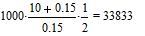 From this value we get the value of the resistor components as:
One loose end from these measurements and simulations is how to apportion Ca1 vs Cg2.
In the time constant of the step settling tests, these two capacitances are calculated as a single capacitance, as they are approximately short circuited by the Ca1g2=85pF internal coupling capacitor. I chose to apportion Ca1=8pf and Cg2=4pF because Ca1 must include the capacitance from A1 to the external shield and is therefor bigger. The proportion between these two capacitors is of little consequence in the two simulations and in the operation of the radio.
18. HF30 RF sweeps
The sparse published data about the HF30 includes a graph to show the dependency of gain in percent variation from peak gain over wavelengths from 200m to 7.5kHz. The graph is unclear in its marking of the longer wavelengths. The spacing of the wavelengths is also odd. The 670m, 2000m wavelengths have a 1:3 space ratio, but 200m which is a little over a third of 670m, should be spaced from 670m about the same, but it is spaced out as if the ratio of 200 to 670 were something like 10:1. I added the corresponding frequency in blue. The AM band lies between 200m and 670m. The vertical scale seems to follow a log spacing. The response at 200m=1500Hz is ~30% and ~75% at 670m=448kHz.
It is also important to note that the source impedance driving G1 and the load impedance at A2 are not specified. Transconductance would be the most generally applicable scale for any load impedance, so the vertical scale might be interpreted as relative transonductance, gm. Transconductance would be measured with a low impedance driving G1 and a low valued resistance loading A2, like 1kΩ.

The following is my own transconductance sweep. I plotted gm in mili-Siemens=mS=mA/V on the vertical linear scale vs frequency in kHz in log scale. In some American literature, Moh was used to represent conductance as the inverse of resistance Ohm. This became obsolete with the assignment of Siemens as the unit of conductance representing Amperes per Volt (A/V). Note that the frequency sequence is reversed with respect to the published graph which represents wavelength in meters.
A brief note about the application of very small signals to the tube inputs: The best practice to avoid external interference, including spurious ground loops, is to set the generator at its highest level, say between 1Vp-p and 20Vp-p and then use a simple resistive attenuator wired very closely to the low level input under test. For example, the generator drives a 10kΩ resistor placed closely to a 100Ω resistor wired directly at the low level input under test. The ground connection of the generator is no longer important as any ground noise is also attenuated by 100x and can be placed anywhere on the ground circuit that is convenient.
My measured peak frequency of 248kHz vs the published 150kHz are in fair agreement, given the very broad peak. My -6dB(50%) at 1675kHz is a better result than the -10dB=30% in the published results. My low end response at 30kHz is -4.6dB=60% is comparable to where 30kHz should be on the curve, but the marked 10000m=30kHz shows about 30%. The low end response depends weakly on tube performance as it is mostly determined by the low cut frequency of the RC coupling network. The R term would include the internal anode resistance in parallel with 33kΩ component load resistor. The internal anode resistance is a function of tube emission, increasing in value with weak tubes.
As we saw in the HF30 DC curve families above, my tubes are weaker than the specification, with gm between 300uS and 800uS, where 1300uS is specified. Even as it is, a peak gm12=3.4mS is very impressive for an RF stage. A strong tube with gm=1.3mS would have gm12=11.5mS as calculated above. The 11.5mS is truly spectacular and would result in a broader bandwidth, as the internal Anode resistance would be 15/1.3mS=11kΩ, instead of 15/300uS=50kΩ with my relatively weak HF30 tubes. The mu=15 factor depends primarily on tube structure and does not change with tube emission.

Comparing with a simulation using my estimated parasitic capacitances and measured gm in my weak HF30 we get:

The following simulation results have a log frequency sweep from 10kHs to 5120kHz. The voltage gain and gm curves are displayed on a linear scale. The dotted curves show the phase in degrees with the scale on the right. The input source has 1Vac, so that the voltage at A1 represents the gain directly. The gm is taken directly from the current flowing through the 0V supply load, which is an AC short to ground.
With gm1=300uS and gm2=800uS as measured above in the DC sweeps we get Gain1=3.9V/V and the combined gm12=2.7mS.
The measured gm12 sweep in the previous figure got a peak gm12=3.4mS. My simulation is a bit pessimistic with gm12=2.7mS, but still close enough to be useful.
Comparing to the simulation from measured values to the simulation with the specified gm1=gm2=1.3mS, we get more than twice the gain on the first stage and nearly 4x higher combined gm12=10.5mS. This is illustrated in the two following simulation results.


Gerhard Einsenbarth says that he has never measured an HF30 that was as good as the specified performance. The cathodes in these tubes were delicate and were used a lot. Finding a very strong HF30 would be a wonderful surprise. One wonders how close to specification a new tube was 100 years ago.
19. 3NFB Anode Bend Detector
The 3NFB employs anode bend detection of the RF signal at its G1 input. The detector operates as a square law detector throughout the signal range, from 12mVp-p to 375mVp-p with a 90V supply and a -500mV bias at G1. Depending on the particular tube, the grid bias can be adjusted for peak sensitivity by a few hundred mV. The optimal G1 bias is also proportional to the HV supply. If the HV supply voltage were doubled to 180V, then the optimal G1 bias would be twice as negative at -1V.
 Square law detection was explored above in the discussion of the architecture at Square Law Detector [3]. The anode bend detector is discussed explicitly and illustrated in Plate bend detector [4].
The figure on the right highlights the square law detection over a wide signal range from 12mVp-p to 375mVp-p of 900kHz RF signal modulated 50% with 250Hz. At 50% modulation level, the carrier is 2/3 of the peak-to-peak modulated signal.
The X and Y axis are in dBVrms.
1V=0dBrms, dBVrms= 20*Log10(VoltsRMS)
The square 10dB divisions in X and Y axis highlight the various curve slopes. The input signal is represented in the horizontal axis ranging from -47.6dBVrms=11.7mVp-p to -17.5dBrms=375mVp-p. It is also represented in the vertical axis in the yellow trace with the expected 45o slope of 1.
| 3NFB-G1 250Hz (dBVrms) | 3NFB-A3 250Hz (dBVrms) | 3NFB-A3 250Hz SFDR (dBVrms) | A3 audio referred to input with gain of 2362, 67.5dB (dBVrms) |
| -47.6 | -38 | -17.2 | -105.5 |
| -41.6 | -25 | -16.9 | -92.5 |
| -35.6 | -12.5 | -18.1 | -80.0 |
| -29.6 | -0.60 | -18.1 | -68.1 |
| -23.5 | 11.6 | -17.8 | -55.9 |
| -17.5 | 23.7 | -17.9 | -43.8 |
Now look at the output blue trace, which has twice the slope with the trace rising by two squares for each horizontal square. Given that the dBVrms scale is inherently logarithmic, the slope of 2 means that the A3 audio output in the blue trace is proportional to the square of the input yellow trace at G1.
The other thing to appreciate is that for smaller input signals the output drops with the square of the input. For example, taking two points from the curve converted to mVp-p, when the input is cut in half from 93.8mV to 46.0mV, the output drops four-fold from 2.64Vp-p to 0.67Vp-p. This relationship also means that the detector becomes ever more insensitive as the input signal drops.
The 3NFB has a measured linear audio gain of 2360x with an audio input and with a 4kΩ AC load at the output anode A3. The AC load means an inductor or transformer load with little DC voltage drop. This gain was measured with a 90V supply. This is impressive for three stages of RC-coupled audio amplification. The bulk of the gain comes from the preamp stages with about 29x for each stage. The last stage only has 0.8mS in the DC curve traces above, as opposed to the specified 1.2ms. With a 4k Load, this gives a gain of 3.2x for the output stage. With overall gain of 2360, the two stages have a gain of 820x and each preamp stage contributes sqrt(820)=29x.
The insensitivity of square law detectors for small signals explains the need for the very high gain of the 3NFB. The green trace is just the blue output trace shifted down by the tube audio gain of -67.5dB=2360x. The gap between the yellow input trace and the green trace illustrates how inefficient a square law detector becomes for small signals. For an RF modulated test input -40dBVrms (28.2mVp-p) on the yellow trace, it would only take only -89dBVrms (100uVp-p) of pure audio on the green trace to produce the same output of -21dBVrms (250mVp-p) at the A3 speaker output. The detection efficiency is only -89dBVrms--40dBVrms=-49dB (0.3%). Even at the highest input level of -17.5dBVrms (375mVp-p) it would take only -43dBVrms (18.3mVp-p) to get the same 23.7dBVrms (43Vp-p), with a detection efficiency of -17dBVrms-43dBVrms=-26dB (4.9%).
 Oddly as it seems, the detected audio is just the distortion signal of the input triode, which is much better as an audio amplifier than as an RF detector.
As was mentioned earlier, the distortion of a square law detector is distortion=modulation/4. For 50% modulation, that is 12.5%, or -18dB. The red trace shows the peak distortion as the Spurious-Free Dynamic Range (SFDR) in the red trace, which follows the -18dB prediction pretty closely, but drops for larger signals as the detection improves beyond square law detection.
The plot on the right shows the blue trace with the output at the A1 anode of the first triode, so that larger input signals can be tested, that would otherwise saturate the two following audio stages. The input range at G1 now extends to 1500mVp-p (-5.5dBVrms) and is shown in the yellow trace. The output at A1 extends to 10dBVrms in the blue trace. The red trace shows the peak distortion (SFDR), which now improves as the input increases above 262mVp-p (-20dBVrms). The DC bias at G1 is -700mV to accommodate the larger input RF signals.
At this point the modulating signal is getting larger than the knee region near cutoff, so that the signal reaches the linear part of the transfer function. See the G1-to-A1 measured DC transfer function in the center plot above. Now with 1500mVp-p at G1, the peak distortion drops to -28dB, which is much better than the -18dB with pure square law detection. This improvement is noticeable while listening.
| 3NFB-G1 250Hz (dBVrms) | 3NFB-A1 250Hz H1 (dBVrms) | 3NFB-A1 250Hz SFDR (dBrms) |
| -5.5 | -28.1 | -28.1 |
| -8.5 | -25.3 | -25.3 |
| -11.5 | -22.2 | -22.2 |
| -14.5 | -20.9 | -20.9 |
| -17.5 | -19.7 | -19.7 |
| -20.6 | -19.4 | -19.4 |
| -23.5 | -19.4 | -19.4 |
| -29.6 | -19.6 | -19.6 |
| -35.6 | -18.4 | -18.4 |
| -41.6 | -14.7 | -14.7 |
| -43.5 | -15.9 | -15.9 |
Anode bend detectors can operate as nearly ideal half wave rectifiers, if the anode bend is sharp compared to the signal to be detected. This requires a larger negative G1 bias and a higher supply voltage. The input signal would also have to be large compared to the turn-off region of the triode. Ideally, the negative peaks keep the triode in cutoff and the positive half of the RF signal brings the triode into conduction and linear amplification. The detecting triode would also be optimized for a lower intrinsic voltage gain mu, around 20. With a 90V supply, the cutoff bias point would be -90V/20=-4.5V and the maximum detectable modulated RF signal would be 9Vp-p. The lower the mu, the more negative the bias voltage and the wider the acceptable input amplitude range. The large signal is also useful to overcome the turn-on knee above the cutoff-voltage into linear amplification. The knee region would be about 0.5V above cutoff for this hypothetical medium mu triode. A high impedance load with a high voltage supply also favors linearity.
Sparks-Withington (Sparton) had a line of radios circa 1930 that used large signal anode detectors. For example, see the Sparton Equasonne 79-A [5]. The detector tube in this AC set was their own C-485 [6] medium mu=12.5 triode, which was also used in the RF amplifier stages. The triode ran with a variable -14V to -20V grid bias and 150V-250V at the audio transformer loaded anode. The variable grid bias also served as volume control. The large signals into and out of the anode bend detector permit it to drive the output tube through an audio transformer.
20. 3NFB Grid-Leak Detector
Comparing Anode Bend detection to Grid-Leak detection: The following is an adaptation to test the 3NFB as a grid-leak detector. The input series resistor RGridLeak1=1MegΩ in parallel with CGridLeak=240pF connected between G1 and the grounded input tank form the grid-leak circuit. The additional RGridLeak2=5MegΩ adds 0.8uA of input bias current to optimize detection. G1 is monitored with a 10x scope probe with 10MegΩ//20pF input impedance.

 900kHz of RF signal from the generator was modulated 50% with 250Hz, driving the variably coupled coil L3. The coupling was kept loose at about a 45o angle. The generator voltage was adjusted to obtain a desired RF level at G1.
| 3NFB-G1 250Hz (dBVrms) | 3NFB-A3 250Hz H1 (dBVrms) | 3NFB-A3 250Hz SFDR (dBrms) | 3NFB-A3 250Hz RTI (dBVrms) |
| -50 | -33 | -18 | -101 |
| -44 | -22 | -19 | -89 |
| -38 | -9 | -19 | -76 |
| -31 | 2 | -19 | -65 |
| -25 | 15 | -20 | -53 |
| -23 | 19 | -22 | -48 |
| -19 | 24 | -25 | -43 |

The grid leak detector modification was inserted under the 3NFB G1 pin. The circuit is wired in with copper tape insulated with a piece of trimmed Dymo label tape. This approach avoids external wiring and interference pickup to the very sensitive G1 input.
The results show pure square law detection for signals from -50dBVrms (10mVp-p) up to -30dBVrms (75mVp-p). Above this level, the loaded input diode that is formed by the grid, cathode and grid-leak resistor starts to sharpen its knee, so that the peak distortion (SFDR) drops to -25dB when the input at G1 reaches -19dBVrms (300mVp-p) and the output reaches 24dBVrms (47Vp-p). With higher input levels, the audio stages start to distort, so we can't increase the input voltage to reduce the distortion further.
Note the slight bent downwards at the top of the output blue curve. Its slope would keep reducing until, when the detection resembles that of an ideal diode with, it acquires the same slope of 1 as the input in the yellow trace for.
The green curve is the output voltage divided by the audio gain of 67.5dB (2360x). As we did with the anode bend detection, the ratio between this curve and the input voltage gives the detection efficiency. With anode bend detection, the input signal (yellow) at -40dBVrms produces produces -21dBVrms at the output (blue), which as an audio amplifier, would require only -89dBVrms. This gap of -49dB shows a detection efficiency of only 0.3%. The same -40dBVrms at the input of the grid-leak detector (yellow) produces -14dBVrms at the output (blue), which as an audio amplifier would require only -82dBVfms. The still very large gap of -82dBVrms--40dBVrms=-42dB presents a 7dB improvement in the grid leak detection efficiency, as compared to the original anode detection result of -49dB.
It is not very surprising that a couple of years later, the Loewe EB100W receiver using the newer 3NFW with unipotential indirectly heated cathodes, used grid leak detection. The other advantage of grid leak detection, is that the detector is operated with maximum current, while the anode bend detection is biased with a low current level. The approximately 0V grid-leak bias makes more RF available at the anode for regenerative feedback. The unipotential cathode also offers a sharper diode knee to improve detection as compared to the softer knee of a filamentary cathode with a 0.8V drop which extends the shape of the knee over this voltage drop.
21. 3NFB with a Germanium Diode Detector
Comparing Anode Bend detection to Germanium Diode detection: Now we further the detection comparison with a Germanium diode detector circuit. The detection is done entirely by the 1N34a germanium diode and the 3NFB is used exclusively as an audio amplifier with G1 biased at -360mV. You will notice two audio attenuators that reduce the detected audio signal by a factor of 4x. The extra resistors make it easy to distribute the smoothing filter over three capacitors C4, C2, C6 with increasing value. The low value of C4=33pF and the relatively light 100kΩ load have a 50kHz corner that guarantees that the AM envelope can be followed without diagonal distortion [7]. Two further low pass filters, keep the audio bandwidth under 3kHz. A wider band filter last filter would have been nicer for music, with C6 reduced to 330pF.


| 3NFB-G1 250Hz (dBVrms) | 3NFB-A3 250Hz (dBVrms) | 3NFB-A3 250Hz SFDR (dBVrms) | 3NFB-A3 RTI 250Hz (dBVrms) |
| -57 | -46 | -18 | -113 |
| -54 | -41 | -19 | -108 |
| -51 | -36 | -19 | -103 |
| -48 | -30 | -19 | -97 |
| -45 | -23 | -19 | -91 |
| -42 | -17 | -19 | -84 |
| -39 | -11 | -19 | -78 |
| -36 | -5 | -19 | -72 |
| -33 | 1 | -19 | -67 |
| -30 | 6 | -21 | -61 |
| -27 | 11 | -22 | -56 |
| -24 | 16 | -26 | -51 |
| -21 | 20 | -31 | -47 |
| -18 | 24 | -38 | -43 |
 The Germanium diode is a fundamentally better detector than any vacuum tube detector because of its much sharper I/V truly exponential curve. The conductance of the diode increases exponentially with voltage drop, as opposed to just 3/2 power function of a thermionic diode. When combined with the resistive load, the germanium diode looks like an ideal diode with much smaller signals than with a thermionic diode. For example, the current flowing and through the Germanium diode and its conductance = 1/impedance double for every increase of 18mV in forward drop. Germanium detector diodes also have a much lower impedance with zero current flowing, on the order of 100kΩ. This makes the diode a pretty good match for the impedance of the tank circuit and no current bias is needed to achieve this impedance, as opposed to the grid-leak detector which requires a forward bias current for optimal detection impedance.
The reason for the 4x attenuator is to allow for larger signals to be applied to the germanium diode detector without the detected audio saturating the audio amplifier. The larger input RF brings the diode into nearly ideal diode behavior.
The germanium diode detector shows a further improvement in detection efficiency. A -40dB input produces a -11dB output. The equivalent audio at the input to generate this level of output is A3-RTI=-80dB. This is a detection efficiency gap of -80dBVrms--40dBVrms=-40dB (1%). But keep in mind that I optimized the circuit with a 1/4x=-12dB attenuator for improved linearity with high input levels. without the attenuator, the detection efficiency improves to 28dB (4%), but this would drive the audio amplifier into clipping.
Summarizing the detection efficiency with -40dBV=28mVp-p at the input is as follows:
| Detector type | Detection efficiency at G1=-40dBVrms | SFDR at A3=24dBrms |
| 3NFB Anode Bend detector | -49dB | -18dB |
| 3NFB Grid-Leak detector | -42dB | -25dB |
| 1N34 Detector without 1/4x attenuation | -28dB | -21dB |
| 1N34 Detector with 1/4x attenuation | -40dB | -38dB |
The germanium detector sounds really sweet at full volume. As became standard in later radios, the volume is always controlled between the detector and the audio amplifier. A volume control with the germanium detector would take advantage of the sensitivity as well as the improved large signal distortion by adjusting the volume control.
22. 3NFB Capacitive Loading at A1
One interesting and accidental finding during my measurements, is that placing the 10x scope probe with 10MegΩ//20pF input loading increased the volume. This actually makes sense. Loading A1 of the anode bend detector with a capacitor, attenuates the Cag1=1pF Miller feedback from A1 to G1 by adding 20pF of additional parasitic capacitance to my estimated internal 16pF.
This effect is confirmed in the following simulation.


 The ".step" command repeats the AC simulation with two values for CA1ext=0 and CA1ext=40pF. This last value is the new capacitor that I added to the radio at the 3NFB-A1 terminal.
I modified the earlier simulations by replacing the ideal input sweep voltage with an ideal input sweep current in I1 and added one of the tank circuits I measured above. The kV scale you see really means kΩ if you divide the voltage by the 1A ideal input sweep current.
This table shows the measured properties of L1 in this simulation. Note the internal 169kΩ equivalent shunt resistance, which be loaded down by G1.
| L (uH) | Fpeak (kHz) | Q | C (pF) | XL (Ω) | Fpeak Res (kΩ) | Coil type |
| 250 | 1132 | 95 | 79.1 | 1778 | 169 | New Litz wire flat waffle |
The first plot shows the simulated response at G1 and its loading effect on the tank circuit. The black curve shows the attenuated result with CA1ext=0 and the blue curve shows the improved signal gain I heard when 40pF was added to A1 as an RF bypass capacitor. Given the very high impedance at A1 around 290kΩ, the 40pF plus the internal 16pF parasitic capacitance form a 10kHz low pass filter. The frequency cutoff is even lower if the loading effect by G2 is included.
If G1 had been biased closer to cutoff with very little DC current flowing, the gm would be greatly reduced, along with the loading effect from Cga feedback.
The second plot shows the loading effect measured in the radio at the L4 socket with the 3NFB tube turned On vs. OFF. The new 250uH Litz wire coil was plugged into L4 and tuned with 101pF to 1000kHz.
The red curve was taken with the power turned off. The gain peak at 1002kHz is 0.0202 with a 12.8kHz BW
The blue curve was taken with the 3NFB turned on. The gain Peak at 1000kHz from the generator to G1 was nearly halved to 0.0119 and the bandwidth nearly doubled to 24.6kHz. With the tank having a measured impedance of 123kΩ at 1MHz, then the input impedance at G1 with the power turned on would be 176kΩ with a simple attenuation calculation.
I also repeated the measurement with 40pF at A1 with 3NFB powered on, as I did in the simulation. The peak gain improved, but only slightly from 0.0119 to 0.0133.
Another variable in the loading effect of G1 is its bias voltage, which I set to -500mV. Changing the bias to -700mV reduces the tube gm and consequently the effect of Cga and the loading presented by G1.
This effect is eliminated with screen grid tubes because their Cga is dramatically smaller, on the order of 0.05pF, as compared to the 1pF in the 3NFB input triode.
23. 3NFB as a very High Gain Audio Amplifier
Audio Distortion: The 3NFB makes a low distortion amplifier, with the dominant distortion at the maximum output of 40Vp-p. The DC voltages are A3=90V, G3=-5.5V, G1=-262mV. The two grid bias voltages at G1 and G3 were optimized for minimum distortion. The A3 output was loaded with a modern transformer driving a modern speaker. The input impedance of the transformer at 1kHz is 8.3kΩ.
 I used the HP3314a function generator to supply the 1kHz test sine wave and a Behringer UCA222 2-channel audio port to capture the output signal. I used Goldwave software to capture the input and output sine waves, and its spectrum display mode to get the peak distortion. I attenuated the signal from the generator by 1001x with a 100kΩ resistor driving a 100Ω resistor load at the G1 input, which is available at the plugin socket for coil L4. This attenuator makes the ground connection of the generator non-critical because any ground interference also gets attenuated by the same 1001x factor.
The UCA222 sound port captured the input through an 11x attenuator made with 10kΩ and 1kΩ into the Left channel from the signal generator. The full scale range of the port is 4Vp-p. The output measurement was attenuated 11x with a 100k and 10k and captured by the right channel. The figure shows an example spectrum with the output at full scale A3=40Vp-p, shortly before it starts to clip softly. I don't recommend using the microphone input of the computer because it could get blown up with an accidental voltage overdrive. The UCA222 is cheap, easy to replace and has a stereo 2-channel input.
The summary of the peak distortion, which is dominated by the 2nd harmonic:
| G1 (mVp-p) | A3 (Vpp) | G1 (dB) | G1 H2-H1 (dB) | A3 (dB) | A3 H2-H1 (dB) | G1 H2 - A3 H2 | Gain (V/V) | Gain (dB) |
| 15 | 40 | -8 | -74 | -3.5 | -30.5 | -43.5 | 2667 | 69 |
| 7.42 | 20 | -14 | -71 | -10 | -36 | -35 | 2695 | 69 |
| 3.72 | 10 | -20 | -65 | -16 | -42 | -23 | 2688 | 69 |
| 1.68 | 5 | -26 | -58 | -22 | -47.5 | -10.5 | 2976 | 69 |
| 0.92 | 2.5 | -33 | -51 | -28 | -52 | 1 | 2717 | 69 |
| 0.92 | 2.5 | -16 | -71 | -28 | -51 | -20 | 2717 | 69 |
| 1 | 2 | 3 | 4 | 5 | 6 | 7 | 8 | 9 |
The voltage measurements in dB are with respect to the audio port full scale of 4Vp-p.
Columns 1 and 2 show the p-p voltage measurements for the input at G1 and the output at A3.
Columns 3 and 4 show the G1 amplitude in dB with respect to 4Vp-p and peak distortion in dB.
Columns 5 and 6 show the A3 amplitude in dB with respect to 4Vp-p and peak distortion in dB.
Column 7 takes the difference between the input distortion at G1 and the output distortion at A3 to make sure that the distortion is much lower at the input than the output. The last two measurements with 2.5Vp-p output, were repeated because the input signal into L was too attenuated by the 11x attenuator and the peak distortion came out nearly identical, so you could not tell if the distortion was at the source or at the output. The 11x attenuator of the input generator into L was removed to show a more accurate version of the same measurement.
Columns 8 and 9 show the gain in V/V and dB at 1kHz with the 8.3kΩ modern transformer load.
3NFB AC response: I performed a classic 3-decade audio log sweep from 20Hz to 20kHz on the 3NFB to obtain its frequency response. The shape of the frequency response was a strong function of the output load at A3. I measured the response with a 4kΩ resistor load, but took care to increase the HV supply to 110V to return the A3 DC voltage back up to 90V for direct comparison with the Inductive loads that have a small internal DC resistance. 4mVp-p was used as the input sweep signal on all the tests
The biggest surprise of the following three frequency sweeps is with the 4kΩ load and its bass peak at 140Hz. With a modern 8kΩ transformer/speaker load, the response was only a slightly modified version as expected as the load was expected to be largely resistive. The third plot shows the response with the Siemens Protos Rfl4 [8] speaker, which has a folded membrane driven by an electromagnetic reed. A reed speaker load is less straight-forward. The second peak in the response at 2kHz can be attributed to the resonance of the 1.3H speaker inductance with the 5nF capacitor at A3 in the 2H3N radio. The switchable 20nF filter capacitor in the speaker was off for this test. The 20nF capacitor would resonate with the 1.3H speaker at 1kHz. The 2kHz frequency peak made the speaker sound crisp as compared with other 1920's reed-&-cone speakers.
| 4kΩ Resistor Load | 8kΩ Transformer Load | Siemens Protos Folded Speaker |
 |
 |
 |
I also made some measurements and calculations of the internal parasitic capacitances to see if I could duplicate the measured response in simulation. Each of the circled components in the following small signal AC simulation schematic represents a triode. The gm and mu were obtained from the published specs [1 p2.35-36]. The explicit component values were obtained from Die Loewe Mehrfachröhren [1 p2.34]. I calculated the three sets of Cga (grid to anode) and Cgc (grid to cathode) values as cylindrical anode-grid-cathode vacuum capacitors with the dimensions obtained from the same source.

The internal parasitic caps Ca1, Cg2 Ca3, Cg3 were estimated from step response tests with a cold tube as was done for the HF30 above.
The following simulated curves are A1 in blue, A2 in Red, A3 in Black. Click plots to enlarge.
The last parasitic capacitor between G2 and A3 is modestly named Cfudge (engineering slang for a guessed value). I selected the value of 10pF which is what gives a simulated bass peak around 200Hz that is similar to the measured sweep with a resistive load at A3.
The simulated 213Hz resonant peak at A3 with Cfudge=10pF is in fair agreement with the 140Hz peak in the measured sweep with the 4kΩ resistor load. I was not able to coax the slight rise in the measured response at 3kHz.
Two plots demonstrate the effect of Cfudge=10pF. The plot on the left has Cfudge=10pF and the plot on the right has Cfudge=0. I also experimented with reducing the gm of the three triodes to half to account for my old tube and it had no appreciable effect on the response shape; reduced gm just lowers the stage gain.
| 20H-20kHz Frequency response at A1, A2, A3 | |
| Cfudge=10pF from A3 to G2 | Cfudge=0pF from A3 to G2 |
 |
 |
I remain suspicious of Cfudge=10pF because it seems relatively high. Perhaps this capacitance is distributed directly between the large A3 anode and the RC coupling network between A1 and G2.
| Peak simulated stage gains at 214Hz | ||||
| Cfudge | A1/G1 | A2/A1 | A2/A3 | Total=A3/G1 |
| 10pF | 40 | 77 | 2.2 | 6800 |
| 0pF | 50 | 50 | 2.2 | 5500 |
Note that this simulation was done with ideal gm and mu as specified for brand new tubes.
The 3NFB specifications: [1 ch3]
24. HF30 Simulated Loading Effect on Input Tank at G1
As we saw with the 3NFB, the input triode of the HF30 has a lossy loading effect on the resonant tank circuit that is tied to G1. The lossy load effect was first illustrated above in section 7. Cga Reflects Anode Load to Grid for the resistive anode load case.
The following simulation compares the loading seen on the resonant tank by G1 with the duplicate unloaded tank at the node "tank". There is also the additional feedback capacitance C_eng_lose that is stepped through the sequence of Cfb values shown in the curve plot. Note that this is the simplified case for Cfb, where it is connected from HF30-A3 to HF30-G1 instead of what is wired in the 2H3N radio, which is from 3NFB-G1 to HF30-G1 and includes the resonant tank at 3NFB-G1.

The following plots compare the simplest case with a 10kΩ load at A2 vs the case where the largest value plugin coil with 2600uH is the A2 load.
The first plot is in log scale magnitude plus linear phase to accommodate the huge peak in the cyan curve. The second plot is in linear magnitude and phase. The two lower plots show the response of a duplicate unloaded tank circuit at node "tank" to compare to the loaded response at G1. The solid curves show magnitude and the dotted curves show the phase.
The phase requires careful interpretation to determine if the circuit is oscillating. The narrowest amplitude peaks show the point at which the combined resistive impedance of the tank tends toward infinity as more and more of the positive resistance losses are canceled by the feedback reflected negative input resistance at G1.
The magenta phase curve in the first plot and the red, cyan and magenta curves in the second plot all show the angle<+90o or angle>-90o (positive real component on the right hand side plane) above resonance in the right hand side of the plots. These high angles indicate a negative (+/-180o) resistive component, which is also close to the real part of the complex impedance in Cartesian coordinates (R+j*X).
One counter-intuitive result is that the magnitude curves that embody a negative resistance, which cause oscillation in the time domain show soft peaks, which suggest limited response amplitude. What does happen is that when the resistive component is negative (angle>+90o or angle<-90o), the oscillation occurs at the soft peak, but the bandwidth of the circuit response also widens as demonstrated by the soft peaks.
You may have experienced this bandwidth widening effect when playing with a radio that has a regeneration control, where you can adjust the regeneration past oscillation while maintaining the oscillation locked to the carrier station with super careful adjustment of the tuning. If you achieved lock, the audio sounds wideband with more treble and there are no oscillation whistles because of the oscillation lock to the carrier. Then, as you reduce regeneration, the audio bandwidth narrows again, on either side of oscillation and the sound is very muffled near the oscillation point.
| A2 Load is 10kΩ | A2 Load is 2600uH//405pF//248kΩ |
 |
 |
Also keep in mind that the load impedance at the anode of the second anode A2 gets reflect to G2, so an inductive load is likely to increase the internal gain with the reflected negative impedance at G2.
25. HF30 Measured Loading Effect on Input Tank at G1
The following 6 plots show the measured loading effect of HF30-G1 on the input LC tank. All plots are in the same log scale for direct visual comparison. The "Kopplung" knob is kept in the minimum "Lose" position. All 6 plots show the signal at G1.
The first plot is for L2=102uH//71kΩ, Q=111 unloaded by turning the HF30 off at the filament switch on the front panel. Note the 9kHz BW and relative peak gain of 0.0225 at resonance from the loose coupled test coil. The parallel 71kΩ resistance accounts for the internal losses of L2.
The second plot shows the dramatic effect of loading by G1 when the HF30 is turned on at the filament switch on the front panel. The gain dropped dramatically by 8.6x to 0.0026. The bandwidth also widened greatly from 9kHz to 67kHz. The tuning capacitor knob would feel to have very insensitive tuning. The apparent input resistance at G1 is 10.3kΩ, which lowers the total resistive loading to 9kΩ. L3=410uH was vertical for minimum coupling to the tuned L4//C3 tank.
Now the third plot shows the untuned L3=410uH coil rotated from the uncoupled vertical position to nearly horizontal for tight coupling to L4, which is fixed horizontally and drives G1 of the next stage stage, the 3NFB input detector. This tight coupling is nearly equivalent to tuning L3 directly. The tight coupling to the tuned L4 tank cancels out the loading at G1, so that the peak gain nearly matches the completely unloaded case in the first plot. However, the response outside the peak, on the skirts of the third curve is still elevated with a loss of selectivity against about 2 channels away at +/-40kHz.
The fourth plot now shows the effect of turning on the 3NFB, which loads its input tank at L4 as shown above in the 3NFB measurements. Now the peak gain at the input tank is about half at 0.012 of what it is with the input tank completely unloaded.
This does show that this operation is oscillation-proof, but with some sacrifice in gain and bandwidth.
All six plots show frequency sweeps at the L2//C2 tank tuned to 1MHz. (click to magnify)
|
HF30 OFF - Unloaded L2=102uH//71kΩ Q=111 |
HF30 ON - Loaded L2=102uH//71kΩ//10kΩ |
HF30 ON - Tuned L4, 3NFB OFF | HF30 ON - Tuned LF, 3NFB ON |
 |
 |
 |
 |
|
HF30 OFF - Unloaded L2=102uH//70kΩ Q=109 |
HF30 ON, L3=2600uH L2=102uH//89kΩ Q=141 |
 |
 |
The first plot on the right is again measured with the HF30 off, but at a different time than the first plot in the row above, so the loose coupling of the test coil is lower and the peak gain is 0.012.
The second plot shows the measured effect of a large inductive load at A2 without coupling to L4. The inductive load should reflect as a negative resistance at G2 and A1 and this increases the internal gain. A1 is tightly coupled internally to G2 with 85pF.
The increased gain of the second plot at G1 suggests that the negative resistance change at A1 ends up getting reflected to G1 as a negative resistance, which reinforces gain and reduces bandwidth.
So, an untuned inductive load at A2 can counteract the loading effect of the HF30 RC-coupled RF amplifier to boost gain and selectivity.
26. Large Signal LTspice Filamentary Triode Models
So far, we have explored the inner workings of the 2H3N DX receiver with small-signal, frequency domain LTspice simulations. We used linear voltage controlled current sources set to the transconductance gm of each triode at the bias point of interest. The intrinsic triode voltage gain mu=μ was modeled with the internal anode resistance Ra, where Ra=μ/gm. Then we added estimated or measured parasitic capacitances Cag, Cgc and Cac, the most important of which being Cag, which makes an undesired feedback path between the anode and the grid, which then greatly changes the input impedance of the grid. We also added a few more parasitic capacitances outside the triodes, that were measured or estimated.
This modeling is fine to explore the linear AC performance of the RF stages in the HF30 and the audio stages in the 3NFB. These linear models are also computationally simple and produce simulation results quickly.
However, the crucial process of RF detection into a low level Audio signal is not possible with linear models. To that end I have created simple non-linear triode models for the identical triodes in the HF30, the two low level triodes and the power triode in the 3NFB. Beyond simulating the RF detection process, these models also model the harmonic distortion in each audio stage.
I based the model on the classic Child-Langmuir diode/triode model that calculates the anode current as a function of grid and anode voltages. This model leaves out the modified behavior in anode current at very low anode voltages (<5V), but we are not going to run the anodes with very low voltages, so this is not a problem. There are other small second order effects on the variation of gm and μ as a function of triode voltages and currents that are not in the model. The primary form of the large signal transconductance law has current as the 3/2 power of the grid voltage plus the 3/2 power of the mu-scaled anode voltage. The 3/2 exponent is also a function of anode, grid and cathode shapes. The ideal case is for a parallel plane triode with a planar cathode, planar grid and planar anode.
 Ia: Anode Current (A)
P: Perveance. It is a scale factor for the strength of the triode (A/V^3/2)
Vgc: Voltage at the grid with respect to the cathode (V)
Vac: Voltage at the anode with respect to the cathode (V)
μ: Intrinsic voltage gain from grid to anode (V/V, unitless)
dA: Diameter of a cylindrical anode (cm)
l: Length of the cylindrical anode (cm)
b: Distance from the anode to the cathode (cm)
I adapted this formula from "Die Loewe Mehrfachröhren" (The Loewe multi-tubes) [1 p2.16] to use the intrinsic voltage gain μ instead of the penetration factor D=1/μ, which was common in early German literature. the 0.00000234 factor for the Perveance calculation came from Die Loewe Röhre 3NFB - Analyse einer Mehrfachröhre [16].
This formula would have been adequate for triodes with indirectly heated cathodes that have a uniform voltage over the entire cathode surface. However, the HF30 and 3NFB have directly heated filamentary cathodes with the necessary voltage drop across the cathode length. In the case of the HF30, the external 4V filament voltage is shared between the two triodes in series so that each cathode sees a 2V variation along its length. In the case of the 3NFB, the two small triodes drop 0.85V each in series with the power triode, which drops the remaining 2.3V for a total 4V of filament voltage.
The primary effect of the voltage variation along the cathode length, is that the sharp anode current cutoff of the Child-Langmuir law occurs gradually across the cathode, with the positive end cutting off first, when the grid voltage is equal to the positive end of the filament minus Va/μ, and then cutting off gradually until the grid voltage matches the negative end of the cathode minus Va/μ, to finish cutting off the anode current completely.
For the 3NFB-V1 at 90V it starts to cut off the positive end of the filament with Vg=0.85V-Va/μ=0.85V-90V/58=-0.7V and finishes cutting off at the negative end of the filament when Vg=Va/μ=90/58=-1.55V.
An ideally sharp cutoff knee with have zero current when the grid voltage reaches cutoff at Vgc<-Vac/μ and conducts with 3/2 power transconductance for Vgc>-Vac/μ.
I created a simple model as a piece-wise approximation of the cathode voltage variation. I used 10 triodes with the anodes and grids in parallel and with each triode carrying 10% of the current. The individual unipotential cathodes are then tied to 10 tap points along a 9-resistor ladder with the total series resistance the same as the hot filament resistance. The summed anode current of the ten triodes has a slight ripple in the transfer curve as each 1/10 sized triode turns on and off sharply according to the ideal 3/2 power law, but this is negligible in our simulation.

Perhaps there is a closed form solution formula for the cathode with a voltage gradient, but I don't know of one. The trouble with integrating the 3/2 power transconductance is that below cutoff the base of the 3/2 power becomes negative and produces an imaginary result with the root of a negative number, but is no problem for LTspice because it rejects the imaginary part and just takes the real part of the result, which is zero below cutoff.
Another advantage of the segmented model with 10 triodes is that any additional voltage drop by the anode current will be seen at the filament resistance series string. In the case of the 3NFB, the effect of the power triode anode current on the order of 10mAp-p will cause several milivolts of filament drop variation where the filament of the input triode connects to the negative end of the preamp triode filament in series with the power triode. This effect causes a negative feedback between the output power triode and the input triode that cuts the overall gain in half.
Now the full simulation schematic with the triode models in the schematic. Each of the TRIODEFIL10 symbols in the following schematic embodies the schematic with the 10 triode segments as a subcircuit.
There are three triode types, the HF30, 3NFB12 and 3NFB3. The parameters [1 p3.45-46 p3.65] of these three triode types are passed along through the symbol with the parameters:
RFIL=16 PER=294.1u MU=15.2 VCT=-0.5 for the HF30
RFIL=6.8 PER=156.8u MU=58.2 VCT=-0.5 for the 3NFB12 preamp triodes
RFIL=18.4 PER=183.75u MU=4.4 VCT=-0.5 for the 3NFB output power triode.
These are visible near the symbols as long vertical or horizontal parameters. They include the total filament resistance RFIL, the perveance Per, the MU and the grid contact potential VCT of -0.5V.

This DC-sweep simulation schematic shows the filaments of each of the triodes in the HF30 and 3NFB wired in series. The voltage source VF2 can be set to 4V at the top of the filament node VF4 to simulate the distributed cathode voltage drop. This voltage can be reduced to 0V to simulate an ideal unipotential cathode. The filamentary cathode resistance of any triode is under 20Ω, so the cathode will still be raised by a few mV at the bottom of the power triode filament, that comes from the power triode anode current.
The two voltage controlled voltage sources E1 and E2 simply scale the grid sweep voltage from Vgrid to 1/4 or to 4x to keep all the anode current cutoff shown in a similar range to the master voltage source Vgrid for easier visualization in the result plots. The anode voltage Vanode is nominally set to 90V, but this value can be stepped discretely or swept in simulation.
Click to enlarge plots

Anode Currents
The plots have a horizontal scale for the master grid voltage V(grid) that extends from -8V to 2V for the HF30 sweeps in the fourth panel. Note that this scale gets reduced 0.25x to -2 to 0.5V for the preamp triodes in the 3NFB shown in the second and third panels, and it is increased 4x to -31V to +8V for the power triode in the 3NFB in the first panel.
Starting with the top panel 1 for the 3NFB_out triode, you see the grid voltage sweep from -32V to +8V in the red curve and the anode current in the black curve. The anode current for positive grid voltages should be a bit less because the grid will take away some of the anode current. This is not a problem for our simulations, because we never simulate strong positive grid voltages.
Panel 2 is for the 3NFB_det with the 3.1MΩ anode load. The red trace shows the grid sweep from -2V to +0.5V. Note how linear this transfer function is for the anode current in the black trace, because such a high anode load resistance looks almost like a pure current source. With a current source anode load, the gain is set by mu, which is a fixed number in our model, so exactly linear, but it usually varies little in a real triode and is thus quite linear.
Panel 4 shows grid currents in linear scale. Panel 5 shows grid currents in log scale.
Panel 3 explores various anode current modes for the two small triodes in the 3NFB as follows:
Blue: 3NFB_pre is reverse biased by the 850mV filament drop of the input triode 3NFB_det, so it has the lowest current level.
Red: Variation in the 3NFB_det filament voltage node V(VFHA) by +110mV from +850mV up to +960mV, as caused by the additional 66mA anode current from the 3NFB_out power triode. (The power triode model current was updated later to have only 37.5% of the current shown in this simulation, so the effect on the vfha node is reduced, but still significant).
Black: 3NFB_det shows the detector current under the influence of a slightly raised cathode voltage up from 850mV to 960mV in the red curve. Raising the cathode voltage reduces the anode current by reducing the effective grid bias, assuming a constant level of emission. Emission (Perveance) variation is not modeled here. Higher voltage on a heater can raise emission and counteracts the bias reduction effect for low frequencies. As we saw earlier in section 14. HF30 and 3NFB Anode Current vs Filament Voltage, the filament voltage has very little effect on cathode emission above a certain voltage.
CYAN: The same type of triode 3NFB_det850mv run independently with a fixed 850mV filament supply. The current is slightly higher than the black curve because it is not back-biased by the extra +110mV. It is a small effect, but can be noticed in overall radio simulation because the overall 3-stage gain is around 6000x (180V supply) and the input triode is a good part of that gain. The feedback from the power triode looks like negative feedback to the input detector triode and cuts the gain to 3000x (180V supply).
MAGENTA: Now we simulate the 3NFB_det0V with zero filament voltage, so that the cathode looks like a unipotential sharp cutoff cathode. All the cathodes in the 10 triode segments in the subcircuit (sub schematic) are now at 0V and they all turn off at the exactly the same voltage which is -Va/mu=-90V/58.2=-1.55V. Note that this horizontal Vg scale is 0.25x, so the cutoff is -1.55Vx4=-6.2V in the horizontal axis. This can't be seen with the real 3NFB because with zero volts at the filament there is no emission. Notice that the current is much higher because there is no distributed 850mV of cathode voltage to debias the triode. There is less curvature in this true sharp cutoff curve than with the triode with the 850mV distributed through the cathode.
 Triode segments and Transconductance
This plot shows the individual segment currents and transconductance of the 3NFB_det850mV triode. Its filament is powered with a fixed 850mV supply, so it is not subject to filament voltage variations from the output power triode.
Panel 1 shows the first triode with its cathode at 850mV, which makes it turn off first at -700mV as seen in the bottom yellow trace of this plot. The last triode to turn off with -1.55V with its grounded cathode is shown in the black trace.
Panel 2 compares the sharp cutoff anode current of the unipotential 3NFB_det0v in the blue curve to the gradual cutoff of the red curve with the 3NFB_det850V that starts turning off at -700mV and finishes turning off at -1.55V, at the same voltage as the sharp cutoff of the blue curve. The upper parts of the two curves have nearly the same curvature while all segments are on.
Panel 3 compares the transconductance (gm) as the slope of the anode current of the unipotential sharp cutoff 3NFB_det0v in the blue trace to the gradual cutoff of the 3NFB_det850mv in the red trace. The extended turnoff region from -850mV to -1.55V is now easier to see in the transconductance curve. You can also see the slight ripple on the red curve that is caused by each of the triodes in the segmented triode model turning off in sequence.
This soft cutoff characteristic is somewhat like a remote cut-off characteristic, except that after the low end of the cathode is cut off, the tube is completely cut off. The cut-off point is stretched over the 850mV range of the filament voltage.
The following plot focuses on the 3NFB anode bend detector.
 We explore here the effect of the 3.1MegΩ resistor load on the anode bend and compare a triode with 850mV drop across its filamentary cathode to a unipotential cathode, with a uniform 0V along the cathode.
Panel 1 compares the anode current with fixed anode current in the blue curve with the sharpening of the knee at V(grid12)=-1.55V and linearization effect of the 3.1MegΩ load which resembles a current source.
Panel 2 repeats the curves in panel 1, but now with a unipotential cathode. The knee at -1.55V is sharpened further in the cyan curve and the 3.1MegΩ load makes the magenta curve look like that of an ideal rectifier.
Panel 3 reexamines the conditions of panel 1, but looking at transconductance. With 90V at the anode we get a near straight line increase in transconductance in the blue trace, which is close to an ideal square law detector. The black trace shows the knee sharpening and linearization of the curve with a 3.1MegΩ load. The flatter the transconductance, the more linear is the current transfer above the knee. The scalloping you see in the black curve is due to the segmented model. The scalloping effect can be reduced by subdividing the triode into more than the 10 segments used in this model. For the specific case of the 3NFB anode bend detector, it would be most efficient to subdivide the bottom 4 triodes into 8 triodes of half the perveance with twice as many filament taps for the 4 extra new triodes. As the black curve suggests none of the top 6 triodes turn off as an anode bend detector with the 3.1MegΩ load and a 90V supply.
Panel 4 repeats Panel 3, but now with a unipotential cathode triode. The cyan curve shows a sharper knee than the blue curve in panel 3. The magenta curve with the 3MegΩ load confirms the nearly ideal rectification of the current, with a very sharp knee and a very flat transconductance.
In conclusion, the high impedance 3.1Meg load greatly improves the anode bend detection of the filamentary triode in the 3NFB. A unipotential cathode would yield nearly ideal anode rectification for large signals.
27. Full AC and Transient Simulation of the 2H3N
Now it's time to have some fun exploring full time domain simulations to dig into some of the secrets of the 2H3N, especially the anode bend detection process and audio harmonic distortion.
This is the first basic simulation schematic with a reference transmission at V(Sender) with 2Vp-p 1MHz modulated by 1Vp-p 1kHz for a 50% modulation. Sender couples to the loop antenna Loop2T with the voltage controlled current source g1, set with a gain of 2.8uA/V, which produces 21mVrms across the input tuning cap C1.
Click the schematic and waveforms to enlarge

The following three schematics model each of the three triode types and are called by the corresponding symbols in the full radio schematic:
triodefil10h.asc for the two HF30 triodes.
triodefil10n12.asc for the two small triodes in the 3NFB.
triodefil10n3.asc for the power triode in the 3NFB.


A few LTspice simulation and configuration notes about the schematic:
- The 3NFB-Ra=3.1MegΩ anode load resistor for the 3NFB-V1 anode bend detector is replaced by a potentiometer of the same value. The following first simulation was done with the pot at full volume to be equivalent to using the fixed load resistor. The purpose of the potentiometer is to try detection of high level signals without saturating the following audio stages. The parameter "Step" can be used to simultaneously change the input signal amplitude and the pot setting when experimenting with a series of simulations using the .step command. The voltage source on the far left side serves to show the Step parameter value after simulation as a voltage, so that it can be probed for the waveform viewer.
- I include the 39pF load at A21 detector anode to improve the detection process and to make the detected audio signal clearer to observe with reduced RF ripple.
- The ESR (Equivalent Series Resistance) and shunt resistance of each inductor are taken from the Q measurements of each coil. I split the Q losses equally between the series and shunt resistances, so that ESR=XL/Q*0.5 and ShuntR=XL*Q*2. If the Q were attributed to either just the series or shunt losses, the 0.5x and 2x factors would be eliminated. The split between ESR and ShuntR could be optimized to match the Q over the AM band. ESR increases losses and lowers Q at low frequencies and ShuntR increases losses and lowers Q at high frequencies.
- The angle of the two variable coupling coil pairs is simulated with the coupling factor K12 L1 L2 0.04 and K34 L3 L4 0.06. Critical coupling for maximum amplitude transfer occurs when K=sqrt(Q1*Q2), where Q1 and Q2 are the quality factor of the two coupled coil circuits. The Q of the L1 tank is a combination of the Q of L1 and the Q of Loop2T. The Q factors for each coil were measured and reported in the table above. This means that if you couple the L1 and L2 resonant coils too tightly the volume comes back down and the selectivity worsens. This is not an issue with L3 and L4 because L3 is not resonated. Optimized the L1-L2 angle for best reception and use the L3-L4 angle for volume control.
- The "Lose - Kopplung - Fest" feedback control is done with CFB and is initially set to zero.
- The heater voltage is set to 4V at +H_4V. Note that the LTspice schematic tolerates different node names on the same wire. This node is also named +H at the multi-tubes . The 4V can be lowered to 0V as an experiment to simulate tubes with unipotential cathodes. Then the current sources G2, G3, G4 automatically reestablish negative grid bias levels for the second and third triodes of the multi-tubes. These supplementary bias sources are off with 4V at the heater.
- C4 C6 C7 are ideal capacitors tied to the heater taps of the two multi-tubes. They are set to zero for the first simulation, but could be set to 1F to simulate the absence of signal coupling from the power triode to the input triodes through these nodes.
- The first simulation shown below was done with the nominal 90V battery. The gain rises substantially with a 180V supply
- The Vdet_Bias source provides a convenient additional source to adjust the grid bias for the 3NFB input detector, It is set to -33mV for the first sim, for a net bias of Vg21=-1.467V
- There is an ideal RF detector tied to G21 with output at G21mag. This is in the two lines of code below the 3NFB.
- The AC simulation includes a calculation of the peak frequency f0, the peak amplitude in dBV, the bandwidth and the equivalent Q, which is the Q that is calculated from the response at a particular stage. For example, V(G21) has the accumulated filtering action of the three resonant tank circuits. The reported Q for V(G21) is not the Q for the resonant tank made by L4//C3.
- The Fourier analysis of the A21, A22, A23 audio voltage nodes is carried out only during the time domain transient simulation and is reported in the .log output file. I report some distortion results the .log files in tables after simulation.
- Al transient simulations first run for 10ms to let all the slow audio time constants settle out before collecting results from 10ms to 12ms. In the context of LTspice, transient means time domain. In the simulations with the 3NF, the settling time was increases to 24ms before saving the last 2ms.
- There is a selection of symbol and schematic downloads at the end of this post in section 50. LTspice Schematic, Symbol and Plot File Downloads
- When you download the two following schematics, be sure to also download all the triodeXXX schematics and symbols that they use and are listed at the end of this post. Rename all the _asc.txt _asy.txt _plt.txt into .asc, .asy and .plt before simulation. These files are all in ASCII format and can be edited directly by an expert.
- The .plt files have a saved preselection of curves to be viewed with particular scales and colors in particular panels. At the end of the simulation, the scale factors are usually on auto-scale. You have to go to wave viewer menus and click Plot Settings>Redraw to import all the save scale settings from the .plt file. This is important on some simulations, because I took the care to select scales to keep the waveforms from overlapping too much. In my installation, the space bar is the hot key to reload the .plt file with its scale factors and also the hot key in the schematics to make the schematic fill the display window. You can set the hot keys by clicking the hammer button for the settings.
- One last display trick for a 4k display: In a lot of simulations I would open an additional blank schematic just to be able to tile the schematic and waveform viewer as three equal vertical columns. I click the wave viewer first, then the schematic, then the blank schematic before hitting the menu Window>Tile Vertically. Then I delete the space holder blank schematic and stretch the left edge of the schematic to the left. Now the schematic occupies 2/3 vertically and the waveform viewer occupies the 1/3 vertically on the right.
28. RF AC simulation from Antenna to Detector
The first simulation is for AC response, and serves to confirm that all three resonant tanks are perfectly aligned at 1MHz, by manually tuning the precise values of C1, C2 and C3.
The input to the HF30 at V(G11) peaks at 75.6dBV/A=6026V/A=6026Ω. This scale is in volts that were generated by the ideal 1A AC source labeled Iac and represents Volts of output per Amps of input, V/A=Ohms, so the vertical scale is transresistance in Ohms. The 75.6dBV represents a slight attenuation of 79.4dBV-75.6dBV=-3.6dB from the voltage across C1 in the first resonant tank that includes the first coil L1 in series with the 4foot-by-8foot antenna loop Loop2T made of two turns of four conductors each, inside CAT5 Ethernet cable.
The input to the 3NFB detector grid V(G21) peaks at 102dBV, for a total RF gain from the HF30 input to the 3NFB input of 102dBV-75.6dBV=26.4dB, which is a total RF voltage gain of 21V/V. Very good for an RF stage in 1926. This raises the detected audio by the square law anode bend detector by 21^2=437x.
Even a modest RF gain of 21x dramatically increases the audio output. So the 2H3N radio is 437x more sensitive than the local receiver version (OE333 [9]) without the HF30. Also consider that no regeneration feedback was used with the Lose-Kopplung-Fest (CFB) feedback capacitor, which can raise gain and selectivity further. In this configuration, this radio is guaranteed free of oscillation! A >400x sensitivity improvement certainly qualifies the Loewe 3H3N as a "Fernempfänger", a DX listening radio!

29. The "Kopplung" control
This is the regenerative feedback control from the third and last L4//C3 tank at the 3NFB detector input to the second tank L2//C2 at the HF30 RF amplifier input. The inclusion of two LC tuned tanks in the feedback loop increases the selectivity for a given percentage of feedback, thus making it easier to get a certain level of selectivity with less feedback, so it is less likely to destabilize into oscillation. See the explanation and simulation of regeneration over one vs two tank circuits at the end of 2-Tank Regeneration [10]. The added internal phase shift in the HF30 complicates the feedback loop further, but the Kopplung feedback control still works very well.

The Kopplung control ranges from "Lose" (loose or light) to "Fest" (tight or high). The rating is from 0pF to 2pF. The following table summarizes the simulation results in the following plots. The gain is represented as the conversion of a current in the loop antenna resonant tank to the voltage at the Loop antenna tuning capacitor C1, to the voltage at the second tank at the HF30 input G11 and to the third tank at the 3NFB input G21.
The first row in the following table is without regeneration with CFB=0pF. The second and third rows are with two moderate levels of regeneration with CFB=0.2pF and CFB=0.3pF. The fourth row is just below the oscillation point with the carefully hand-tweaked value of 0.375pF. The fifth row marked in red is with too much regeneration and the circuit oscillates with CFB=0.5pF.
| Loop Antenna tank at C1 | Second Tank L2//C2 - G11 | Third Tank L4//C3 - G21 | |||||||
| transresistance (kOhms) | (KHz) | (Hz/Hz) | transresistance (kOhms) | (KHz) | (Hz/Hz) | transresistance (kOhms) | (KHz) | (Hz/Hz) | |
| CFB (pF) | peak_c1 | bw_c1 | Q_C1 | Peak_g11 | BW_G11 | Q_G11 | Peak_g21 | BW_G21 | Q_G21 |
| 0 | 9140 | 46 | 22 | 6026 | 33 | 30 | 126678 | 17 | 60 |
| 0.2 | 9830 | 43 | 23 | 12757 | 10 | 96 | 256507 | 9.0 | 111 |
| 0.3 | 11414 | 35 | 29 | 28691 | 4.2 | 240 | 560919 | 4.1 | 245 |
| 0.375 | 169064 | 0.355 | 2824 | 326400 | 0.354 | 2838 | 6262533 | 0.354 | 2837 |
| 0.5 | 23502 | 7.3 | 137 | 20828 | 5.3 | 188 | 389000 | 5.2 | 193 |
The peak values are for the peak voltage that is generated from a 1A ideal current into the loop antenna resonant circuit. This transfer characteristic is called transresistance in V/A=Ω units. You can find the voltage gain by dividing the transresistance value at a voltage node by the transresistance value at another voltage node. The third panel shows the transresistance gain at the 3NFB G21 detector input. The solid values are the magnitude of the transresistance in Ohms and the dotted curves are the transresistance phase.
Finding oscillation in an AC simulation is tricky, because the magnitude response softens again as seen in the magenta curves for the input at V(g11) in the second panel. You have to look for a sudden phase change that does not follow the pattern of the phase before oscillation. The phase change marks oscillation in the magenta curve of the center plot.
The teal (green-blue) curve is on the verge of oscillation with CFB=0.375pF. As expected, it offers a very high additional gain of 49x as seen in the third plot, but also extremely narrow bandwidth of only 354Hz, which barely lets any audio through. Also note that regeneration works by increasing the signal at the input V(g11). The gain of the HF30 does not change with regeneration.
One property of all regenerative receivers that regenerate the signal into the antenna circuit, as this set does, is that the regenerated signal boosts the RF near the antenna and is beneficial to other radios tuning the same station. But if the regeneration breaks into oscillation, then you will get a whistle in other radios, as the regenerative oscillation is usually not synchronous with the carrier. This is to be avoided.

 The plot on the right gives further insight on the effect of regeneration.
You will noticed that the overall gain of the two inverting stages in the HF30 RF amplifier is nominally non-inverting, except for additional phase shifts that occur inside the HF30 and at the resonant L4//C3 tank.
The non-inversion suggests an opportunity for neutralization.
Neutralization is the concept of adding feedback through an additional capacitor, but with a non-inverted version of the signal, to neutralize the negative feedback through Cga. Neutralization uses positive feedback through a capacitor. Neutralization is achieved by selecting a feedback capacitor value and positive gain that match the negative feedback through Cga.
The positive feedback is usually obtained by taking signal from the opposite end of the resonant tank that causes the undesired negative feedback via Cga. This ensures that both paths have identical frequency response, but opposite signal polarity.
It seems that the "Kopplung" capacitor provides nominally positive feedback, but the frequency response of the HF30 and the resonant L4//C3 tank alter the frequency response of the positive feedback. This plot immediately above compares the response of the input tank at node V(g11) under three different conditions:
Black trace: The HF30 filament power is OFF, so there is no significant loading of the input circuit. The coupling level is critically coupled.
Blue trace: The HF30 filament power is ON and the attenuation by about 0.5x with reduction in selectivity is clear to see.
Red trace: The HF30 filament power is ON, but CFB has been increased to 0.2pF to bring the response at 1MHz approximately the same as it was the the HF30 turned off.
This is similar to neutralization, but not quite the same, because the frequency response outside 1MHz is quite different from the unloaded case with the power turned off.
In any case, a small amount of feedback via the Kopplung capacitor CFB, can eliminate the loading effect at the resonant frequency and offer additional selectivity. Increasing selectivity beyond the unloaded Q of the resonant tank would not be the result of true neutralization. True neutralization just restores the unloaded response of the LC tank.
You can take a deep dive into the topic of Neutralization at RF Amplification with Triodes [17] by Dr Rudolf Cantz 1953. The original German text of this PDF was translated to English in collaboration with me and RM members Dietmar Rudolph and Hans Knoll.
30. Transient Simulation of RF, Detection and Audio
This first full time domain simulation shows the full progress of the modulated signal from across the input tank formed by the loop antenna Loop2T in series with L1 resonating with C1 at V(ant1,ant2)=3mVrms to the output at the Siemens Protos speaker at V(a23)=9.1Vrms on the right side of the schematic.
The overall voltage gain from the input to the HF30 RF amplifier at V(g11)=2.42mVrms to the output of the 3NFB detector at V(a21)=171mVrms is 70.7x.
The audio gain from v(a21)=70.7mVrms detector through the audio amplifier in the 3NFB to the Siemens Protos Rfl4 speaker at V(a23)=53x.
The combined RF and Audio gain is 3760x. 4.3mVrms of 50% modulated RF at the HF30 input produced 12Vrms at the speaker.
The overall power gain from the input tank at V(ant1,ant2)*I(L1)=8.4nW and the speaker terminals at V(a23)*Ix(3nfb-v3:A)=22mW is 22mW/8.4nW=2678000 = 64dB.
The speaker signal magnetizes a reed between the poles of a magnet that drives a folded diaphragm. The high frequency reproduction of the Siemens Protos RfL4 speaker is quite good. Some paper cone speakers of the period sound muffled or very resonant at a particular frequency.
Each RMS voltage value for each signal is compared to the signal of the previous stage and the stage gain is shown as a multiplier. The overall reference level is the signal at the HF30 input V(g11)=3.4mVrms - 1x.
The progress of the signal is shown through the radio in each panel. The waveform names refer to labeled voltage nodes a labeled pin currents in the schematic. Note the first appearance of the detected audio signal at the anode labeled a21 of the first 3NFB triode in the black trace of the 5th panel. The RMS detector gain from RF at the input grid g21 to the anode a21 is only 2.4x. If the input were an audio signal the stage gain would be more like that of the audio preamp at a22 with an audio gain of 34x instead of just 2.4x. This low square law detection efficiency from the RF at g21 to the audio at a21 is consistent with the real measurements shared above.
The distortion levels at 1kHz were copied from the .log output file and pasted in the center bottom area of the schematic. They are also marked in panels 5, 6 and 7 of the waveforms.
V(a21) = 171mVpeak, THD = 10.1%
V(a22) = 5.2Vpeak, THD = 3.5%
V(a23) = 9.1Vpeak, THD = 7.3%
Some of this distortion improvement could be due to Audio bandwidth limitations we measured above that filters out some of the harmonic content. But it seems more likely to be due to some distortion cancellation accumulated through the audio stages.

31. Audio-Only AC simulation
The following schematic is modified by turning off the 1Amp RF AC source on the left and introducing a 1V Audio AC source at V(G21_Bias) and set the bias at G21_Bias to -0.5VDC. These are the only changes to the previous schematic.
You can find the corresponding simulatable schematics, symbols and plot command files in section 50. LTspice Schematic, Symbol and Plot File Downloads. Rename the file extensions as directed.
You can change between AC and transient audio operation by editing the modifications shown here, where the antenna signal on the left is disabled and audio is injected by the vdet_bias voltage source driving G21.

The following results show the bandwidth limitations and also the very high gain of 65.6dB=1905x from the input of the 3NFB at V(g21) and its output at the speaker terminals V(A23). The final bandwidth is gradually reduced from 4.2kHz at the input of the preamp triode V(g22) to the output with a 2.1kHz bandwidth at V(A23). The main high frequency limitations are due to the internal 3NFB parasitics at the very high impedance internal nodes and also due to the 5nF filter capacitor at the 3NFB output. The output in the red trace for V(A23) at 2kHz is only 2.5dB down from the value at 1kHz, so filtering was not the main reason why the distortion was reduced from the detector output to the speaker terminals in the time domain simulation for the full radio.
There is a further interesting effect at the filamentary cathode taps in the 3NFB. These are V(K21K22) for the input triode and V(k22k23) for the preamp triode. Very surprisingly there is a gain of 2dB at 100Hz from the input to the first triode's filament as seen in the magenta trace. This signal is placed there by the filamentary cathode of the output triode, which is in series with the two smaller triodes. the phase profile is non inverting in the blue dotted curve, so that means that this signal at the filament represents negative feedback from the power triode filament to the input triode filament.
The second plot on the right shows an additional simulation with 1Farad bypass caps at K21k22 and K22K23 to bypass any feedback from the power triode to K21k22. The feedback to K22K23 is larger, but that tap is for the second triode with one less stage of gain to the output. The labeling on the right plot is for the unbypassed simulation as is shown in the left plot. You can see the slight difference of behavior in the additional superimposed curves.


32. Audio-Only Transient Simulation at 1kHz
Now the transient simulation schematic is modified by turning off the signal into the antenna at the G1 voltage controlled current source by multiplying its gm factor by zero. Then set the bias at G21 to the middle of the linear range at -0.5V and apply 16mVp-p (5.6mVrms) sine wave with the Vdet_Bias voltage source into G21. The distortion results and audio signal levels are shown at the bottom of the schematic.

The following plots show a 5mVrms 1kHz sine wave at the input V(G21), then amplified 29x to 144mVrms by the first triode at V(G22). The second stage amplifies this 33x to 4.8Vrms at V(G23). The power triode gives the final 1.8x voltage amplification to 8.75Vrsm. The overall audio gain is 1750x.
This 1750x gain is only half of the overall gain of 3760x for the full radio from the RF input LC tank at G11 to the speaker terminals at V(A23). The RF amplifier in the HF30 makes up for the very low detection efficiency of the anode bend detector.
The sine waves look much cleaner here than those that come from the detector above. The harmonic distortion is much cleaner as shown at the bottom of the schematic immediately above. The total harmonic distortion at 1kHz is 2.2% at V(A21), then 5.5% at V(G23) and 4.6% at V(A23) speaker terminals.
The output current through the power triode is shown in the blue trace as 2.3mA RMS. Most of this current flows to the +H filament terminal and some 0.67mArms flows down the power triode filament to the filaments of the two other triodes. This 1kHz current causes 4.1mVrms voltage drop at the top of the preamp filament at node K12K22 in the green trace of the third panel. We already determined that the gain from the first triode to the output is 1750x, so the 4.1mVrms appears as negative feedback at the first triode that is driven with 5mVrms at its input V(G21). This seems like it would be a significant cancellation, but keep in mind that the first triode cathode is distributed along its filament so only approximately half of the 4.1mVrms, or 2mVrms, affect the anode current of the first triode.
I stepped the simulation with a 1F bypass capacitor at K12K22 to eliminate the 4.1mVrms there, and the gain variation for the input stage increased only slightly ass seen in the plot on the right. This is a modest effect because only the upper part of the filament of the first triode affects the anode current. The effect is more significant with a 180V supply because the stage gains approximately double so the anode current at the output doubles and increases the 1kHz feedback into the K21k22 node.


33. Optimize the Bias Voltage at the Detector Input
The square law characteristic of the anode bend detector in the 3NFB-V1 is not perfectly uniform. The detector grid bias can be optimized for maximum volume and for least distortion. The grid voltage to anode current characteristic of the anode bend detector was modeled in section 26 Large Signal LTspice Filamentary Triode Models. The 3NFB detector plots at the end of section 26 shows a nearly straight line increase of transconductance with increasing grid voltage, given a fixed 90V anode voltage. But the anode bend detector is loaded with a 3.1MegΩ load that linearizes the transfer function as you increase the voltage past the -1.55V knee. This was observed in section 12 3NFB Measured DC Curve Families with the measurement of A1 current vs input grid voltage with the 3.1MegΩ anode load tied to a fixed 90V supply. See the yellow trace in the plot for the 3NFB-NEW sweep.
I repeated the transient simulation with a series of values at Vdet_bias that bias the G21 detector input in the 3NFB. The input to the detector at G21 is 227mVp-p (80mVrms). The following table shows the sequence of bias levels at G21 and resulting amplitude and distortion. These were generated by the .fourier statement and were obtained from the .log file.
The distortion results in the table also show that the detection curve is not uniform and not perfectly square law. The expected distortion from 50% modulated RF is %distortion=%modulation/4, 50%/4=12.5%, or -18dB.
RF at V(G21)=300mVp-p (106mVrms)
| G21 bias (V) | A21 (mVpeak) | THD at A21 (%) | |
| -1.6 | 45 | 16 | Detector is cut off |
| -1.5 | 162 | 9.1 | Lowest distortion |
| -1.3 | 241 | 10.1 | Highest output level |
| -1.1 | 240 | 10.7 | |
| -0.7 | 210 | 13.4 | |
| -0.3 | 45 | 9.3 | Attenuated by grid G21 conduction |

 The first panel in the plot shows the modulated RF input to the detector. The RF input at G11 is 6.1mVp-p. The amplified RF input at G21 is 227mVp-p, which is small enough that it will be detected with square law detection.
The sequence of colors is the same for all 3 panels and they start with black, blue, red, etc, as seen in the first panel. Note how the input to the detector at G21 gets attenuated when the bias is -0.3V in the top brown curve. The G21 grid starts to conduct at -0.5V, so at -0.3v, the input was attenuated by more than half.
The next panel shows the detected 1kHz audio at the input of the preamp triode G22. These values would normally be superimposed because the input bias at G22 is fixed at ground. The effective bias is -0.85 because the cathode of the preamp triode is in series above the detector triode. I added the value of the DC bias level for the detector to these curves to separate them and make it easier to identify them after they are AC coupled to G22.
The third panel shows the output detected audio A23 driving the speaker. The highest level is within a few Vp-p of the maximum level without clipping. (The voltage swing at the speaker is high, because the perveance for the power triode was 490uA/V^1.5 instead of the more accurate 184uA/V^1.5 that was found after the simulation).
The black trace in the second and third panels show no detected audio with the -1.65V bias because the detector is completely cut off. The most sensitive bias level is with G11 biased to -1.3V, as seen in the fourth trace colored in cyan.
Note the second harmonic distortion is noticeable on all the traces with the tops of the detected 1kHz flattened somewhat. This is to be expected from the square law detection.
34. A Wide Range of RF Input levels
Now we are going to vary the input level at the HF30 input in 5 attenuating steps of 0.5x from 24.4mVp-p down to 1.525mVp-p. The DC bias at the detector G21 is selected from the previous set of curves as optimal at -1.3VDC. The 3.1MegΩ variable volume control at anode A21 was kept at maximum to match the real 3.1MegΩ load inside the 3NFB multi-tube.
The arrows point to the spice commands that repeated the curve family 5 times.
You can find the corresponding simulatable schematics, symbols and plot command files in section 50. LTspice Schematic, Symbol and Plot File Downloads. Rename the file extensions as directed.
This time I increased the integer parameter Step from 5 to 9 to change the input level at the input voltage controlled voltage source as a negative exponent. The current into the loop antenna starts at 1.4uA and decreases with 0.5x attenuation steps down to 87.5nA. The reason for the decreasing amplitude sequence is so that the smaller amplitudes will display over the initial larger amplitudes. The first panel shows the Step parameter sequence with the first largest signal shown in the black curves. The smallest signal is shown in the magenta curve. The same color sequence applies to all panels.

 The following table shows the anode bend detection at A21. The RF amplitude decreases in 0.5x steps, which, with square law detection, results in the detected audio at A21 decreasing in 0.25x steps.
Note the increased distortion to 17% at the highest level of 508mVp-p at the G21 detector input. At this level The positive peaks are large enough to start being detected linearly, while the lower RF levels remain closer to square law. That causes the flattening in the positive peaks of the detected black trace. At this large level a more negative bias level would have improved the distortion. An extra simulation with 508mVp-p at G21, but with -1.5V detector bias gave 13% distortion.
| Step | Into Loop (uAp-p) | G11 (mVp-p) | G21 (mVp-p) | A21 mVpeak | THD |
| 8 | 2.1 | 10 | 284 | 239 | 12% |
| 9 | 1.05 | 5 | 142 | 65 | 7.2% |
| 7 | 0.53 | 2.5 | 71 | 18 | 10.5% |
| 8 | 0.026 | 1.25 | 35.5 | 4.1 | 10% |
| 9 | 0.013 | 0.612 | 17.8 | 1.03 | 9.7% |
Improving the distortion for the highest of these levels with 508mVp-p at G21 is not useful, because the high detected level causes the output amplifier to clip at A23 speaker input. The square law detection and the 0.5x makes the output amplitude change by 0.25x for each step. Panels 4 and 7 scale the signals with increments of 4x to display all the simulations at a similar level.
35. Add a Volume Control for Large Signal Detection
One of the fundamental developments in the evolution of radio design was to move the volume control from the RF stages to the audio stage input. This was usually accompanied with some sort of automatic RF gain control to guaranty that the strongest RF inputs did not saturate the RF stages. This allowed for the RF signal amplitude at the detector to be optimized for the lowest distortion with a strong detector input. Any remaining audio level variation was handled by the audio volume control.
Some radios have a very effective AGC that also keeps the audio variation from station to station at a minimum into the volume control input, so that you don't need to change the volume control setting when you change stations. Typical 5-tube American AC/DC radios that I am familiar with, have an AGC that works fine to eliminate RF distortion, but is poor at regulating volume level between weak and strong stations. See Detection and AGC in a 5-tube AC/DC radio for more on AGC.
I replaced the anode bend detector load resistor with a 3.1MegΩ audio volume control after detection. to see how the detection distortion could be reduced with higher RF levels at the detector.
You can find the corresponding simulatable schematics, symbols and plot command files section 50. LTspice Schematic, Symbol and Plot File Downloads. Rename the file extensions as directed.

 This time, the Step parameter decreases the input by 0.5x scale factors while the volume control increases its setting by 4x factors. Steps 5 to 9: 0.00156x 0.0625x 0.25x 1x 1x. Keep in mind that above 0.25x, the 4.8MegΩ bias resistor for G22 causes additional attenuation. This reduces volume variation, while driving the 3NFB anode bend detector with the maximum possible signal of 2.08Vp-p into the 3NFB input grid at G21, as the first simulation step. As we can see the THD at A21 (detector anode )and A23 (speaker) in columns 6 and 8, the smaller signal levels are still detected with square law detection, while the larger signals improve detection toward ideal rectification.
As the table shows, the output volume at the speaker terminals A23 remains fairly constant from step 6 to step 8 as the 0.5x attenuation steps at the input are matched with opposite 4x volume increases.
| Step | RF Into Loop | RF at G11 | RF at G21 | Audio at A21 | THD | Audio at A23 | THD |
| uAp-p | mV | mVp-p | Vrms | % | Vrms | % | |
| 5 | 16.8 | 77 | 2080 | 9.1 | 3.8 | 8.1 | 1.9 |
| 6 | 8.4 | 38 | 040 | 3.67 | 4.8 | 12.2 | 5 |
| 7 | 4.2 | 19 | 520 | 1.26 | 6.9 | 14.3 | 7.1 |
| 8 | 2.1 | 9.6 | 260 | 0.24 | 10.1 | 12.9 | 7.3 |
| 9 | 1.05 | 4.8 | 130 | 0.056 | 12.8 | 3.3 | 10.1 |
| 1 | 2 | 3 | 4 | 5 | 6 | 7 | 8 |
The amplitude of the black trace with the highest RF level of 2.08Vp-p at G21 is smaller because it no longer follows the square law detection. The last curve in magenta with the smallest RF level of 130mVp-p is diminished because the volume control was maximized in the previous step to full 1x gain. The two smallest curves have the same volume setting of 1x.
The greatly improved distortion shows the advantages of having a volume control after the highest possible RF amplification that the detector can tolerate.
36. How much Better is a Unipotential Cathode Detector?
 The voltage drop across the filamentary cathode of the input detector triode in the 3NFB softens the cut-off characteristic of the triode. Ideally, this anode bend detector would have a perfectly linear fixed gain above cutoff and zero gain below cut-off. The transitional region is the so-called "anode bend". A unipotential cathode triode would have a much sharper "anode bend", because its cutoff voltage would not be extended over the entire 850mV drop at the filamentary cathode.
The calculated plot shows anode current in μA vs grid voltage on the horizontal axis. The curves are repeated for fixed anode voltages of 45V, 90V, 135V and 180V. The unipotential triode curves in red contrast their sharp cutoff with the very gradual cutoff of the blue curves for the distributed filamentary cathode of the 3NFB anode bend detector.
Keep in mind, that it is likely that the cutoff of a unipotential cathode may be not as sharp as shown here in the red curves. One possible reason for the slight smearing of the cutoff point is variations in the control grid spacing throughout the grid spiral length. These variations affect Durchgriff=1/mu directly, which controls the cutoff point of the triode directly. Simply stated, the cutoff grid voltage is Vgoff=Vanode/mu. The grids in the following photo have uneven spacing, but this may have been caused by their removal. There is also the "Inselbildung" (island formation) effect, which is the uneven emission under grids that are close to the cathode. When the grid is close to the cathode, not only does cutoff stop current from flowing through the grid, it actually reduces cathode emission directly under the grid wires. This will start reducing current disproportionately, before cutoff, thus rounding off the cutoff point. In any case, even with second order effects, a unipotential cathode has a sharper cutoff than a filamentary cathode.
Gerhard Einsenbarth had these comments on spiral grids in the translated "The Loewe Muilti-Tubes" page 2.42
 "The left image: 2.101 shows the two grids of an older 3NF. The differences in the dimensions of the grids of the power amplifier (top) and preamplifier (bottom) are clearly visible. The grid of the power amplifier triode is plain and the grid of the preamplifier triode is blackened. The more tightly wound grid requires greater heat dissipation, which is provided by the blackening. The grid lengths of both grids are slightly larger than the respective lengths of the anode in order to prevent so-called wrapping. The lower left photo, image: 2.102, shows the grids of the two preamplifier triodes. The upper grid is from an older version of the 3NF and the lower grid is from a newer version with an internal metal shield. The slight differences in pitch and diameter lead to differences in the penetration value, so that the lower grid has a smaller penetration value and thus enables the triode to achieve higher amplification. Such changes/optimizations to the triodes during production are not documented by Loewe."
It is trivial to change the nature of the cutoff in simulation using the segmented triode model shown above in section 26 Large Signal LTspice Filamentary Triode Models. To simulate the distributed voltage drop on the filamentary cathode, you drive the 3NFB with its rated 4V filament voltage. For the unipotential cathode simulation, you simply set the filament voltage to 0V. This works in simulation because the triode perveance and emission in simulation are not functions of the filament voltage; only the gradual cutoff is affected by the filament voltage drop.
The following three schematic thumbnails repeat the three previous transient simulations that had 4V at the filaments, but now with 0V at the filaments and 1Farad bypass capacitors at the filament taps to block the feedback from the power triode 3NFB-V3 to the anode bend detector at 3NFB-V1.
Click schematics and plots to enlarge
| Sequence of Bias Levels | Sequence of RF Levels | Sequence of RF Levels & Volume control |
|---|---|---|
 |
 |
 |
Each of the following 3 tables compares the previous results with +H=4V at the filament with the results with +H=0V and 1Farad bypass caps at the filament taps to simulate a unipotential cathode. The RF input at G21 is noted in mVp-p. The detected audio is compared at the anode bend detector anode A21. The fundamental amplitude at 1kHz is marked with H1 in V and the second harmonic is marked with H2 in %. The higher order distortion H3, H4, etc is negligible.
Sequence of Bias levels at the detector grid G21 with -1.55V, -1.5V, -1.4V, -1.3V, -1.2V for +H=0V.
| +H=4V |
G21 RF 300mVp-p |
+H=0V |
G21 RF 100mVp-p |
|||
|---|---|---|---|---|---|---|
| Vdet bias | A21 H1 | A21 H2 | Vdet bias | A21 H1 | A21 H2 | |
| V | Vpeak | % | V | Vpeak | % | |
| -1.6 | 0.045 | 16 | -1.55 | 0.091 | 13.4 | |
| -1.5 | 0.162 | 9.1 | -1.5 | 0.193 | 3.3 | |
| -1.3 | 0.241 | 10.1 | -1.3 | 0.063 | 11 | |
| -1.1 | 0.24 | 10.7 | -1.1 | 0.041 | 10.9 | |
| -0.7 | 0.21 | 13.4 | -0.7 | 0.026 | 11 | |
| -0.3 | 0.045 | 9.3 | -0.3 | 0.0063 | 11. |
The te st signal for +H=0V is a relatively small 100mVp-p. The less sensitive filamentary cathode above with +H=4V required 300mVp-p for comparable output at the anode A1 of the detector.
The detector triode cutoff is -90V/mu= -90V/58.2= -1.55VDC. The optimal bias point is close to cutoff for a unipotential cathode shown on the right in blue. The stepped bias sequence revealed -1.5VDC in the blue curves in the following plot on the left to be the optimal bias level with a fixed 100mVp-p RF at the G21 detector input.
Sequence of RF levels. The detector bias is now set to the optimal -1.5V for the unipotential cathode with 0V at the filament.
| +H 4V |
VDetBias -1.2VDC |
+H 0V |
VDetBias -1.5VDC |
|||||
|---|---|---|---|---|---|---|---|---|
| Simul. | G21 RF | A21 H1 | A21 H2 | Simul. | G21 RF | A21 H1 | A21 H2 | |
| step | mVp-p | mVpeak | % | step | mVp-p | mVpeak | % | |
| 8 | 284 | 0.239 | 12 | 10 | 100 | 0.193 | 3.3 | |
| 9 | 142 | 0.065 | 7.2 | 11 | 50 | 0.061 | 9.6 | |
| 10 | 71 | 0.018 | 10.5 | 12 | 25 | 0.013 | 10.3 | |
| 11 | 35.5 | 0.0041 | 10 | 13 | 12.5 | 0.003 | 9.3 | |
| 12 | 17.75 | 0.00103 | 9.7 | 14 | 6.25 | 0.00076 | 9.2 |
The input RF am plitude at the loop antenna is stepped in half factors. After amplification by the HF30, the RF level at the G21 detector input is 100mVp-p, 50mVp-p, 25mVp-p, 12.5mVp-p and 6.25mVp-p. The highest of these levels gives a full scale speaker output of 30.1Vp-p in the Black curve below in the center plot.
The input sequence is in factors 0.5x, but the levels at the speaker output are scaled in the viewer in steps of 4x, starting with a 1x level in the black curves. After this 4x step scaling the levels are all similar, thus confirming square law detection. This square law combined with the 0.5x RF input level sequence gives the 0.25x audio level sequence.
Sequence of RF levels & volume control. I activated the virtual volume control at the detector anode that replaces the 3.1Meg load resistor.
| +H 4V |
VDetBias -1.2VDC |
+H 0V |
VDetBias -1.5VDC |
|||||||
|---|---|---|---|---|---|---|---|---|---|---|
| G21 RF | A21 H1 | A21 H2 | Pot | G21 RF | A21 H1 | A21 H2 | Pot | |||
| step | mVp-p | Vpeak | % | 4^(Step-8) | step | mVp-p | Vpeak | % | 2^(Step-11) | |
| 5 | 2080 | 9.1 | 3.8 | 0.01563 | 6 | 1500 | 7.72 | 2.4 | 0.03125 | |
| 6 | 1040 | 3.67 | 4.8 | 0.0625 | 7 | 750 | 3.44 | 2.3 | 0.0625 | |
| 7 | 520 | 1.26 | 6.9 | 0.250 | 8 | 375 | 1.52 | 2.2 | 0.125 | |
| 8 | 260 | 0.24 | 10.1 | 1.000 | 9 | 187.5 | 0.652 | 2.1 | 0.25 | |
| 9 | 130 | 0.056 | 12.8 | 1.000 | 10 | 93.8 | 0.255 | 3.4 | 0.5 |
 The volume increases in steps of 2x in the sequence (0.03125x 0.0625x 0.125x 0.25x 0.5x) as the RF input drops in steps of 0.5x in the sequence (1.5Vp-p 0.75Vp-p 0.375Vp-p 0.188Vp-p 0.094Vp-p).
The volume was at maximum in the previous 2 simulations to match the real fixed 3.1MegΩ load inside the 3NFB. With the volume control, I was able to increase the RF level into the G21 detector input from 100mVp-p to 1.5Vp-p. This increase in amplitude brings the detection out of square law region and toward ideal rectification. This is particularly true for unipotential cathodes, as the low distortion levels show in the table on the right, where the worst distortion is 3.4% when the detector RF input level is at its lowest with V(G21)=93.8mVp-p.
The output signals at the speaker terminals A23 in the third panel are not scaled in the viewer, because the volume control was already adjusted during the simulation in a sequence of 2x steps up to 1x full volume level.
If the detection with high input levels were ideal, the variation in input RF level would correspond exactly to the same variation in detected audio level. The third panel with audio at the speaker shows that the smallest input level has dropped behind the volume adjustment by about 50%, but this is still not square law detection, where a 16:1 attenuation from the black curves to the magenta curves in the RF levels at the detector input G21 would correspond to a 256:1 variation in detected audio output.
There is also the second order effect, that the 4.8MegΩ bias resistor at G22 will load the tap of the 3.1MegΩ and attenuate the 0.5x volume level below 0.5x, thus attenuating the magenta curve more than the other curves. The loading effect diminishes at lower volume levels as the output resistance of the potentiometer is reduce toward zero, as the volume is reduced toward zero. The sharp cutoff of the unipotential cathode reduced distortion in the detected levels, as they got out of square law detection and into linear rectification with smaller RF signals.
37. Operating the 2H3N as an OE333
The operating instructions of the 2H3N DX receiver also include the option of turning off the HF30 RF preamp with its filament power switch and feeding the antenna signal directly into the 3NFB Detector and Audio amplifier. In this configuration, the antenna drives L3 with variable coupling into the fixed L4 coil which is tuned by the variable capacitor C3 (30pF-560pF). In Germany, this type of radio that uses only one tuned LC tank circuit is known as an "Einkreiser"- (single circuit). Radios in Germany were marketed from early on and into the 1960's, by the number of tuned LC tanks in the signal path. The LC tank used in the local oscillators of superheterodyne sets does not enter into the count.
 In this configuration, with one tuned LC tank and using only the 3NFB multi-tube, the radio becomes equivalent to the contemporary Loewe model OE333 from 1926, shown here on the right in the nice photo from Wikipedia. The "OE" means "Ortsempfänger" - (Local receiver). With the filament power to the HF30 turned off, the output antenna ties to A0 and ground to E0 on the lower right of the front panel in the 2H3N receiver.
Local receivers were popular in Germany from the 1920's and into the early post-war period, when resources were scarce. These include the very widely produced "Volksempfänger" by many makers in several variants during the 1930's, like the DKE "Deutscher Kleinempfänger" - (The small German radio). One of the very last "Einkreiser" radios was the very pretty Grundig Gloria 51GW from 1951/1952 [11]. Receiving just one or two local stations was a viable market in this period. Some of he "Einkreiser" radios had two sets of coils, or a tapped coil, to tune the MW (550kHz-1500kHz, 545m-200m), also known as the AM band, or the LW (~150kHz-300kHz, 2000m-1000m) band, but still with one tuned tank on either band.
The Wikipedia photo shows the OE333 with the original 3NF multi-tube with thoriated filament. The 3NF preceded the 3NFB, which had a much higher emission Barium coated filament.
The OE333, like all "Einkreiser", was expected to be operated with an outdoor long antenna, but if close enough to the station, an indoor antenna would be enough.
I set up the following simulation as closely as I could to the intended use, which was with a single tuned LC tank and a typical outdoor wire antenna between 15m (50ft) and 30m (100ft). My good late friend and former RM member Dr Dietmar Rudolph has an excellent German language post on dummy antennas [12] that look electrically like a real receiving antenna when driven by a bench generator. You could use an on-line translator if necessary. I copied the circuit from the post showing the standard antenna from the IRE (Institute of Radio Engineers in the US) in 1948, which works from 150kHz to 30MHz. The dummy antenna is shown in the dashed box. It has a nominal impedance of 360Ω∠-60o at 1MHz. The ∠-60o angle indicates a lossy capacitive impedance. A pure capacitance has ∠-90o angle.
You can find the corresponding simulatable schematics, symbols and plot command files section 50. LTspice Schematic, Symbol and Plot File Downloads. Rename the file extensions as directed.

The dummy antenna was actually quite good to experiment with and select the antenna coil with a number of turns that gave the best performance. I started out with a 241uH coil from the table in section 2. Plug-in Coils because it looked like it had a similar number of turns to the coil shown in the OE333 photo, which may have had 50 turns. Loewe identified coils with the number of turns marked on the coil plugs.
This coil turned out to be not as good a choice as the 102uH coil, which corresponds to 25 turns. The smaller coil gave a better impedance match and when the coupling angle was adjusted for the same RF level at the tuning LC tank. The better impedance match also resulted in better selectivity with a 26.8kHz bandwidth shown here, vs a less selective 38.1kHz bandwidth with 241uH coil (not shown here). I'm very pleased that the simulation with the IRE 1848 standard dummy antenna gave me an idea of the operation of the OE333 if I had a long outdoor wire antenna.
Note that the antenna circuit is not tunable and shows a broad peak toward the low end of the band at 700kHz. The broad width of the peak is expected from the relatively high antenna radiation resistance modeled by the 400Ω and 200Ω in the dummy antenna circuit.
The time domain response on the right shows the same detection behavior as the 3NFB with the full 2H3N, but with higher input RF levels to make up for not using the HF30 RF amplifier, to get a full speaker volume output.
Note how the L3-to-L4 variable angle coupling was adjusted in K34 L3 L4 0.1 to get optimal response. At this coupling level, the sensitivity was quite flat over the MW (AM) band, with less than a 3dB (100% to 70%) variation as you tune over the entire 500kHz-1500kHz range. But even this can be tweaked with the coupling angle and the coil value. The 25 turn coil gave optimal results with the long wire dummy antenna.


38. Operating the OE333 Configuration with a Large Indoor loop Antenna
I have for decades now used large indoor loop antennas instead of long-wire outdoor antennas. Their sensitivity is adequate even for crystal radios to receive local stations. As mentioned above, I used a 4-foot by 8-foot (1.2m by 2.4m) rectangular loop with this 2H3N radio. It works just as well in the single stage "Einkreiser" in OE333 configuration.
I took advantage of the presence of the three tuning capacitors and coil sockets in the 2H3N radio to configure my OE333 with a tuned loop antenna in series with L3 and C1 with variable coupling to the L4//C3 tank driving the input of the 3NFB multi-tube. This additional tuned LC tank makes for a "Zweikeiser" (two circuits) radio.
The following schematic marks the 2 necessary jumpers shown in magenta for use with a loop antenna as shown in the schematic, or with an external long wire antenna. The "Kurz-Lang" switch is still active. As before, this rewires the tuning cap in parallel or in series with the loop antenna and the coupling coil L3. Be sure to keep the power switch the HF30 filament off, if the HF30 is in the socket. Otherwise, the A2 anode will load down the tuned L3 tank. This configuration is actually better than the OE333 because now the antenna circuit is also tuned with high Q to improve sensitivity and selectivity. With the two tune LC tanks, this is now a "Zweikreiser".
One note about LTspice simulation: All circuits must eventually have a path to ground shown in the little upside-down triangle symbol attached to a wire. The letter G brings up the ground symbol for attachment to a wire. If you use an independent LC tank that couples to another coil via a Kxy Lx Ly CFactor, you must also add a ground symbol to the LC tank for the LTspice simulation to run and avoid the "matrix singularity" error, which just means the existence of a completely floating circuit.

39. Adding a Notch Filter to the OE333 Configuration
The 2H3N DX receiver came with three tuned LC tanks. We just used the first and third tuned LC tanks to configure an improved OE333 with two LC tanks as a "Zweikreiser". We can apply the unused second L2C2 tank as a variable notch filter. This is a flux absorption notch filter, because it is only inductively coupled to the antenna circuit via L1. There is no direct connection to the antenna circuit. This floating circuit is convenient, because in the OE333 configuration, the Loop antenna circuit sits at 82.5VDC in the anode load circuit of the unused HF30 and the L2C2 tank sits at -1.5V bias of the unused HF30 input.
A variable notch filter is useful to attenuate a strong local transmitter, so you may be able to receive a weaker station that is relatively close in frequency. These filters were usually optional circuits in German "Einkreiser" radios with a single LC thank. My Grundig Gloria 51GW Einkreiser from 1952 [11] came with a location in the plastic chassis to mount an optional notch filter. Notch filter in German is "Sperrkreis" (choke circuit).
The L2C2 tank has the variable capacitor to tune its frequency and the variable coupling angle to control the notch effect on the L1 coil. In the previous circuit with two LC tanks, we had a jumper at L1, but now we put it to good use with the 25 turn 91uH plug-in coil.
 For the first example I picked a notch frequency that is at 934kHz below the 1MHz signal of interest. For the second example I with picked a notch at 1146kHz. The 2 plots below show the transfer function from the injected ideal 1A AC current into the loop antenna to the antenna voltage (Ant1-Ant2) across the tuning capacitor and to second tuning LC tank at the detector input G11. The output units are Volts/Amp=V/A=Ohms. The upper panels are in log scale and the lower panels are in linear scale.
Note in the two plots below how the spurious peak that comes with the notch is below the notch if the notch is below the desired frequency (left plot) and it is above the notch if the notch is above the desired frequency (right plot).
 I include the slightly different schematic on the right for the higher frequency notch filter case with the different values for C2 and the readjusted loop antenna tuning capacitor C1. Click on the small schematic to see the C1 and C2 values for the notch above the frequency of interest.
The depth of the notch is controlled by the angle of the L1-L2 coils, which sets the L1-L2 coil coupling factor K12, which is 0.3. Below this value the notch depth is reduced. More coupling degenerates the effect. Tuning the notch filter requires retuning the antenna until in the end the notch is tuned to the interfering station and the loop antenna is tuned to the desired station. The notch tuning and the antenna tuning are interactive.
The maximum attainable notch depth is a direct function of the Q of the L2C2 notch tank.
The notch on the left has rejection of 1/139x (43dB). The notch rejection on the right is 1/207x (46dB). This is very effective in killing my local station at 680kHz to make it easier to hear a weaker station at 740kHz.


It is possible to place a series-connected resonant tank in the antenna circuit, but that requires an external coil and tuning capacitor that are not part of the 2H3N receiver. This external tank would be a normal tank, connected to the antenna circuit via a low tap in the resonant notch LC tank. A step-down separate winding with about one quarter of the turns would also work and would provide galvanic isolation.
40. Notch Filtering in Transient Simulation
The transient (time domain) simulation of a signal at 930kHz modulated by 3kHz interfering with the desired 1MHz modulated by 1kHz shows surprising results, which is that in AM envelope detection in the presence of two RF signals of different amplitudes, the stronger of the two signals suppresses the weaker signal beyond the suppression of the linear LC notch filter. This suppression effect in AM detection [13] is well illustrated in the German language post by Dietmar Rudolph. This simulation confirms the suppression effect by the stronger station on the weaker station.

The two following time domain results (click to enlarge) show the transmitter's (Sender) desired 1MHz-x-1kHz desired signal in black and the interfering 930kHz-x-3kHz in red on the first panel of both plots.
The second panel of the left figure shows 6uArms (cyan) of the desired 1MHz signal and 95uArms (red) of the interfering 930kHz signal injected by the G1 and G4 voltage controlled current sources (transconductors) respectively. The notch filter and the resonant loop antenna clean out a lot of the 930kHz interference as seen at the RF input to the 3NFB in black as the current through L3 in series with the loop antenna.
The third panel shows the notch filtered result as a voltage across the loop antenna tuning capacitor C1. Now we see the 3kHz envelope (6 cycles in 2ms) of the interference at a similar level to the 1kHz (2 cycles in 2ms) of the desired signal.
The fourth panel shows the additional filtering of the signal by the third tuned tank at L4//C3. Now the 1kHz is very prominent with a residual level of 3kHz.
After detection, the 3kHz signal is no longer visible in panels 5, 6 and 7. Panel 6 is a bonus panel which show the result of an ideal absolute value detector of the signal at G21. This ideal detector shows zero distortion of the 1kHz and no 3kHz interfering signal at all. This proves the integer rejection concept with an ideal envelope detector. Also note how similar the 3kHz suppression is between the anode bend detector in panel 5 and the ideal detector in panel 6.
The right figure steps the amplitude of the 930kHz interfering antenna signal in seven halving steps from 128x higher than the desired 1MHz signal down to 2x of the desired 1MHz signal. See the gm expressions in the G1 and G4 transconductors:
G1=2^(3)*1uApeak=8uApeak
G4=2^(4 to10)=16uApeak to 1024uApeak .
Note that at the 64x higher interference, it is barely noticeable in the audio curves at the bottom in blue. It takes a 128x signal at 930kHz to finally get clear 3kHz in the audio output, but even then the interfering 3kHz riding on the desired 1kHz is substantially less than the 1kHz signal.


41. Comparing Anode-Bend to Grid-Leak and 1N34 detector in the OE333
The simplicity of the OE333 configuration also lent itself to compare the built-in anode-bend detection with grid-leak (Audion for German readers) detection and with Germanium diode (1N34 diode type) detection. See the related experimentation and simulations above. The following schematic shows the three detection modes in sequence. Having these three configurations in the same simulation schematic makes it easy to compare their performance under the same conditions. The shaded magenta boxes highlight the differences between the detector configurations.
All three detector configurations have 2.6uArms of modulated 1MHz RF current into each of the loop antennas at Loop1, GLLoop1 and L5. Note that each loop antenna and series tuned capacitor on the far left is in series with a 25-turn plug-in 91uH coil, that plugs into the adjustable right-hand side variable coupler in the L3 location of the radio. So the loop antenna resonant tank consists of the loop antenna in series with the coupling coil and the tuning capacitor.

Before proceeding further into time domain simulations that show the detection process, I manually tweaked the values of all 6 tuning capacitors to resonate precisely at 1MHz to produce the AC response curves shown here.
 The first panel shows the voltage response across the tuning caps of the loop antenna circuits for all 3 versions. Black curves for the original anode bend detection version (OE333 detection), blue for the second with grid-leak detection and red for the third with germanium diode 1N34 detection. The result is shown in dB, but it really means Volts of response for 1A of ideal injected loop antenna current. The dB is directly convertible to a transresistance. For example 78dB means a transresistance of 7.9kV/A=7.9kΩ. The AC simulation is perfectly linear, so using 1A as the input current to the loop antenna is convenient for the V/A transresistance math.
The dip at the center of the loop antenna curves in the top panel is caused by the loading of the second tuned tank circuit that drives the detectors. The black curve for the anode bend detector circuit is slightly less attenuated because the anode bend detector grid poses very little active load as it is biased near cutoff. The blue curve for the grid-leak detector shows the heaviest loading on the loop antenna tank, as its grid is intentionally forward biased and loads the second tank slightly, with only an additional 2dB attenuation in the red curve at 1Mhz, as compared to the black anode bend detector curve.
Also note the coupling factor between the antenna circuit coil and the detector circuit coil as expressed by K12 L1 L2 0.04 for the first detector is different than the K12GL GLL1 GLL2 0.06 and K121N L1_1N L2_1N 0.04 for the other two circuits. I had to tweak these coupling factors because of the different loading conditions for a similar response. In the real circuit, you would turn the variable coupler. Also keep in mind that maximum coupling between to high-Q resonant tanks occurs at a particular angle and the signal decreases with tighter coupling, as we saw above in section 3 The Coil Coupling Angle between High-Q Resonant LC Tanks.
The second panel shows the overall response from the Loop antennas to the 2nd tuned tanks driving the detectors. The different bandwidths for the three circuits show a narrower, more selective bandwidth of 32.5kHz for the anode bend detector in the black curve vs nearly 50kHz less selective bandwidth for the grid-leak and Germanium diode detectors in the nearly coincident blue and red curves.
The response of the OE333 shown above with just one tuned LC tank and an untuned dummy long wire antenna has skirts like those of the loop antenna in the first panel and the peak shape of the black curve of the second panel. The original OE333 configuration is substantially less selective than when using the two tuned circuits.
 Now that the three sets of LC tanks are perfectly tuned to 1MHz, we can look at the time domain simulation results to appreciate the detector performance for each case. The curves follow the same color convention from panel to panel.
Blue: Anode bend
Red: Grid-leak
Blue: Germanium 1N34
The first panel shows the relatively small signal of 80mVp-p. that appears at the antenna tuning capacitor. The second panel shows the stepped up 120mVp-p undetected RF input to the anode bend detector in the black curve, with mix of RF and detector audio at the grid-leak detector input for the red curve and the fully detected audio from the 1N34 Germanium diode in the blue curve. In the case of the 1N34 detector, the 3NFB works strictly as an audio amplifier.
The grid conduction is modeled as a simple thermionic diode without any effect from the anode voltage. I practice, the Anode voltage reduces input grid conductance. But in this case, the forward bias of the grid leak detector pulls the DC voltage at the A21_GL anode down to 50V, which would help detection in a real radio. It is possible to include the effect of the anode voltage in the grid diode model, but I did not do it here. With the high mu of the input triode, the effect of the anode voltage on the grid conductance is greatly reduced. Compare this to the low voltage that is required with detector triodes with the low mu=8, as is the case of the contemporary ubiquitous American tube 01A, which required the anode voltage to be reduced to between 22.5V and 45V for sensitive detection.
The third panel shows the signal at the anode of the first triode in the 3NFB, where all three radios have a detected 1kHz audio signal. Note how much stronger the 1N34 detected signal is. Some of this is because the input triode is operated at maximum gain as an audio amplifier. The grid of the power triode G23 starts to conduct at about 0.5V below the +1.7V at low end of the power triode filament voltage. So the third triode grid will conduct above +1.2V. The positive peaks stay below -1V, so no trouble here.
The fourth panel shows the final THD distortion values for each path at the speaker terminals A23. It is surprising to see the grid leak distorting less than the 1N34. Perhaps the distortion improvement is the result of some 2nd harmonic cancellation with the forward bias operation of the grid-leak detector. The distortion of the black and blue curves is close to the 12.5% distortion prediction that was calculated during the experiments above as Distortion=Modulation/4. 50% modulation yields 12.5% distortion.
The most sensitive detector is the 1N34 in the blue curve with 24Vp-p, then the grid-leak detector puts out 10Vp-p and the anode bend detector is least sensitive with only 6Vp-p. This disparity was seen in the real radio above during the experiments with these detector configurations.
42. Using the External A1 terminal in the 3NFB
The external A1 terminal (here A21) at the anode of the first triode of the 3NFB makes it possible to add low impedance load resistors. This makes it possible to check the detector performance with higher RF input levels and avoid hard clipping at the audio stages with higher detected audio levels. The solid magenta arrows point to the three load resistors, that I added in parallel with the internal 3.1Meg anode resistor at A1. This raises the maximum detectable RF level to 1.2Vp-p at the second tuned tank driving the three detectors. The 3 load resistors are 50kΩ, 20kΩ and 15kΩ respectively, for each detector.
As expected, the original less efficient anode bend detector requires higher gain with the 50kΩ load than the other two detectors. I also added 500pF detection filters at A1. With the low load impedances, the internal parasitic capacitance at A1 is no longer sufficient to filter out the RF from the detected audio.
Unlike with the imaginary volume control replacing the 3.1Meg anode resistor in earlier simulations, the external loads at A1 can be used in a real experiment. The only disadvantage of the low impedance load resistor is that the linearization effect for the conduction part of the anode bend detector that we saw in the 1st and 3rd panels of the last plot of section 26 (Large Signal LTspice Filamentary Triode Models) is lost. With the low impedance load, the transfer function is close to the blue curves of the 1st and 3rd panels.
The 1.2Vp-p is the largest voltage that the anode bend and grid-leak detectors could tolerate without saturating the detection process. As seen above, in the 1N34 detector experiments, the 1N34 detector could detect much higher voltage levels, with the only limitation being the reverse breakdown voltage of the 1N34 around 50-75V, but I wanted a direct comparison here for high level detection between detectors, so I injected the same 29μArms into each of the three loop antennas.

The color convention remains the same in the various panels for the plot: Black for anode bend detector, blue for grid-leak detector and red for 1N34 germanium diode detector.
 The first panel shows the loop antenna tuning capacitor voltage around 800mVp-p. This level is similar to what I get from my local 50kW AM station 5 miles away with my large 4ftx8ft loop antenna. This represents typical local receiver "Ortsempfänger" conditions. The second panel shows the voltage stepped up by the coupled LC tanks to 1.2Vp-p at the input of the detectors. Note the three different bias levels at 3NFB-G21 input: Anode bend at -1.3VDC near cutoff, Grid leak near 0V and 1N34 detector at -0.6 for audio amplification only, without detection.
The third panel shows the detected anode bend current at A1, the detected RF+audio at the grid-leak grid G21 and the fully detected audio by the 1N34 at grid input.
The detected audio in the envelope of the red trace at the grid of the grid-leak detector shows a THD of only 1.3%. The THD at the 1N34 node is only 0.7%. These two very low levels of distortion illustrate the advantage of large RF signal detection with 1.2Vp-p amplitude.
Panel 4 shows the first anode A21 for all the detected audio signals around 0.5Vp-p. The low value of the load resistors keeps the DC value near 90V. Some second order distortion is visible on all three curves because a relatively large range of the input grid voltage is being used, which extends into the gradual grid cutoff over the 850mV filament power drop. Even the 1N34 signal gets distorted at the anode to 8.5%, which is noticeable in the blue curve, but still worse in the other two curves: Anode bend is 10% and grid-leak is 15%.
The distortion of the amplified 1N34 signal at the A1 anode could have been reduced by attenuating the audio into the 3NFB with a volume control, while keeping the 3.1MegΩ high impedance load to linearize the triode gain. In the experiments above I tried a 0.25x attenuator in the real radio, after the 1N34 and got -38dB SFDR (Spurious-Free Dynamic Range), which corresponds to 1.2% distortion at the speaker terminals. It sounded very nice!
Panel 5 has the grid drive for the power triode at G23 and confirms that the positive peaks stay below grid conduction that starts when the grid reaches the power triode cathode voltage of +1.7VDC (2.3V filament drop - 0.5V grid contact potential).
Panel 6 shows the result at the speaker terminals. Distortion changes through the stages and can even cancel somewhat because the distortion is mostly 2nd harmonic. The power supply is at 90V, but the peaks exceed 100V because of the inductive load.
The following table summarizes the distortion results for this simulation in line 3 and then with reduced RF at the detector in lines 4, 5 and 6 as shown the column 2.
Column 3 lists the external load resistors at A1 and columns 4, 5 and 6 shows the detector distortion.
The last line is with half the RF input shown above, down to 660mVp-p. The external load resistors were increased as shown in column 3 to get the output up to the original levels of line 3. This reduction of the signal in half with higher gain gave the best results for a ~30Vp-p output swing.
Increasing the load resistor reduces the distortion of the input triode as an audio amplifier. That is evident in the distortion improvement between A21 the anode bend detector at on the last line in green. The load at A21 was increased 7x to 350kΩ.
The distortion for the 1N34 audio output is quite good on line 6 and is limited by the distortion of the audio the second audio preamp and the output power triode. THD at A21_1N=1.0%, A22_1n=5.6%, A23_1N=4.1%. Curiously enough, the distortion at the 1N34 detector is 3%, but it gets somewhat canceled by the distortion of the first triode, so that the distortion at A21_1N=1%.
| STEP | RF | R13 R8 R12 | A21 | G21_GL | 1N34 | A23 | A23 | A23_GL | A23_GL | A23_1N | A23_1N |
| mVp-p | kΩ | % | % | % | Vpeak | % | Vpeak | % | Vpeak | % | |
| 4 | 1320 | 50 20 15 | 9.9 | 1.3 | 0.7 | 15.1 | 10.1 | 14.2 | 11.5 | 15.1 | 7.2 |
| 4.5 | 930 | 50 20 15 | 10.2 | 0.9 | 1.5 | 8.6 | 9.7 | 13.7 | 6.6 | 13.0 | 4.1 |
| 5 | 660 | 50 20 15 | 11.2 | 0.5 | 3.0 | 4.58 | 10.5 | 11.5 | 3.6 | 9.87 | 2.8 |
| 5 | 660 | 350 30 22.5 | 7.7 | 0.6 | 3.0 | 16.0 | 7.6 | 15.6 | 4.3 | 14.0 | 4.1 |
With a higher voltage supply, like 180V, all the distortion values would have been better as all the cutoff points of all triodes would have doubled, thus allowing larger signals to be detected for the same internal loading configuration in the 3NFB. I saw this improvement while making my distortion measurements in the real radio.
43. The 3NF Multi-Tube in the First Version 2H3N
I based all my LTspice tube models above on my HF30 and 3NFB multi-tubes that came with my 2H3N Radio. I followed published specifications and my own measurements to create the models.
I present here an attempt at a pair of models for the 3NF with thoriated cathode filament, which was the first version of the 3NFB with sublimated barium cathode filament. One 3NF model was created for the two small triodes and one 3NF model for the power triode. I used the published curves as the basis for the large signal models. I don't have a working 3NF, so I kept the parasitic capacitors the same as what I measured for the 3NFB. The 3NFB is a fully compatible upgrade to the 3NF, but keep in mind that the internal layout of the two tubes is quite different so the my reuse of the 3NFB parasitics for the 3NF is a compromise. Click the following plots to magnify.

 The red curves show the model curves superimposed on the original data sheet curves.
One of the problems with both tubes, is that the cutoff is even softer than what my models, with their segmented filamentary cathode, can predict.
Could the cutoff softening be caused by the island effect (Inselbildung), where the space charge is suppressed directly under the grid wires? Could it be caused by variation in the pitch of the grid spiral, where the tighter turns cut off before the wider turns? Could it be an end effect where the cutoff at the ends of the filament is often more remote?
In the case of the small preamp triodes shown on the left, it was enough to lower the exponent of the anode current from 1.5 to 1.3 to bet a good overall fit, except for the cutoff that is still more remote in the specified curves in the left plot.
In the case of the power triode shown on the right, I had to parallel a lower mu=3 triode to the main triode with mu=5 to get the very remote cutoff to be anywhere close to the published curves. The fit is good enough to be useful in simulations, because the nominal operating point with a 90V HV supply is with -7.5V at the grid, which is in the most linear part of the curve. This is even less of an issue with a 135V HV supply, as the operating point is that much further from cutoff and the grid bias is also 50% more negative. In the following simulations I found the optimal bias for G3 to be -9V with a 90V HV supply and -12V with a 135V HV supply.
Both curve plots show the new values for the filament resistance (RFIL), perveance (PER), intrinsic voltage gain (MU) and new exponent (EXP) parameter for the the anode current formula.
The two schematics show the simulation schematic for the 3NF preamp on the left and the simulation schematic of the 3NF power triode. Note that two triodes in parallel were necessary on the right to account for the relatively remote cutoff of the power triode in the 3NF multi-tube. One triode has a mu=5, which dominates the behavior in the linear region. The other triode has mu=3 to extend the cutoff toward the cutoff of the published curves.
The resistor and capacitor values inside the 3NF were taken from "Die Mehrfachröhren" [1, p2.38]. This includes the recommended use of the 135V high voltage supply. The following two schematics generated the red curves that were superimposed above on the original data sheet curves.
| 3NF preamp triodes with 2V series filaments | 3NF power triode in two parts |
 |
 |
The sub-circuit hierarchy for the 3NF power triode starts with the schematic above right and continues below. The symbol 3NFOUT in the 0 schematic above right is marked below with 1. This symbol points to the subcircuit schematic 3NFOUT of the compound triode in 2. Each of the two triodes TRIODEFIL10exp in 2 have different parameters that are passed down to two instances of the schematic TRIODEFIL10exp in 3.

You can use the 3NFOUT.asy symbol to replace the TRIODEFIL10N3.out in all the schematics above. If you do that, you will need to connect the 4V filament of the 3NFOUT.asy between ground and the 4V source. You will also need to update the parameters of the two preamp triodes with the parameters shown in the first schematic. The preamp triodes have their 2V in series between the 4V supply and ground.
You can find the corresponding simulatable schematics, symbols and plot command files in section 50. LTspice Schematic, Symbol and Plot File Downloads. Rename the file extensions as directed.
The following two plots show the transconductance on the top panels and the anode current in the bottom panels. The left plot is for the 3NF preamp triodes and the right plot is for the 3NF power triode.
The transconductance (gm) for the 3NF preamp triodes on the top-left shows the effect of the segmented filamentary cathode. This is more pronounced for the 3NF than for the 3NFB, because the 3NF has 2V across its filamentary cathode, which spaces each cathode in 200mV steps, while the 3NFB has a 850mv filamentary cathode and each cathode segment is spaced only in 85mV steps.
The transconductance (gm) for the 3NF output triode on the top-right panel shows a strong kink that is caused by paralleling the two triodes with m=5 and mu=3. If you zoom in, you will also see a vestige of cathode segmentation, which has the cathode segments spaced in 400mV steps. The reason why these coarse steps are barely noticeable in the gm curves is because the mu is very low, between 5 and 3.


The following schematic shows the Loop antenna version of the OE333 modified for simulation with the 3NF.


The first simulation is the AC response to ensure that the the loop antenna tank with L1 and C1 and the detector tank made with L2 and C7 are both aligned to 1MHz. I had to tweak C7 by a couple of pF when I replaced the 3NFB with the 3NF.
Now the response is virtually the same with 32.3kHz bandwidth, as compared to 32.5kHz simulated earlier with the 3NFB.

 It took some experimentation with the input G21 grid DC bias and the output G3 grid bias for maximum swing capability without clipping. Both of these bias levels are direct functions of the HV supply. The plots on the right show the transient simulation with a 90V and a 135V HV supply.
The new schematic above shows on the lower right two ".param" statements that select the bias voltages and input signal amplitude for operation with a 90V or a 135V supply. You just comment out the unused parameter set with an *. This makes it easy to switch supplies quickly.
1.07Vp-p of modulated RF at G21 produce 18.9Vp-p with 10.7% distortion at the A23 speaker output. This compares with the earlier result from the 3NFB, where 284mVp-p of modulated RF produces 25.2Vp-p 1kHz output audio. Each of the stages in the 3NF is less sensitive, starting with the input anode bend detector. The 3NF als has the further disadvantage of have more than twice the voltage drop at the filament, with 2V vs 850mV. This softens the cutoff more than twice as much.
Note that the internal coupling caps in the 3NF are 1.5nF, which is about double the value of the coupling caps in the 3NFB. This slowed down internal time constants, which required a long initial time domain simulation of 24ms before saving results for the last 2ms. With the 3NFB in the earlier simulations, a 10ms internal settling time was enough before saving the last 2ms. I also added the Gstart current step at the start of the simulation, to counteract the initial disturbance of the starting RF detection at the start of the transient simulation that appears across the first 1.5ns coupling cap C2. The Gstart starts the simulation with 371nA and drops to 0nA during the first us.

The key difference between the first generation 3NF and the later 3NFB is the lower gain and power output for the 3NF.
The schematic and plot on the right show the audio frequency response with a 20Hz-to-20kHz audio sweep at the G21 input. The input was biased for linear audio amplification with the bias set in the third .param with -1V.
Note the much smaller peak AC audio gain of only 335x (50.5dB) at 632Hz for the 3NF. This compares to an audio gain on the order of 2000x for the 3NFB.
The following schematic and plot show the time domain audio response, along with the distortion at each stage, G22, G23 and A23. The overall THD at the output A23 is 3.4% with a 17.5Vp-p voltage swing and a 90V supply. Note that the RF signal from the L1//C7 tank was disconnected for the audio simulation. The audio signal source is at the center of the schematic.

You can find the corresponding simulatable schematics, symbols and plot command files in section 50. LTspice Schematic, Symbol and Plot File Downloads. Rename the file extensions as directed.
44. The 2HF Space Charge Tetrode Multi-Tube in the First Version 2H3N
 The original version of the HF30 RF amplifier multi-tube, with two triodes, was the 2HF with two space charge tetrodes. At the moment I don't have a suitable LTspice model for the space charge tetrode. The original published curves for the 2HF are on the left.
Space charge triodes were used in the mid-1920's to boost gm with thoriated tungsten filaments. A higher gm lowered the impedance of the overall RF circuit to widen bandwidth and increase gain.
The grid closest to the filamentary cathode was tied to a modest positive voltage, like 21V for the 2HF to neutralize the space charge and make more current available. The second grid was then used as the input control grid.
After the introduction of the more emissive barium coated filaments and unipotential cathodes, no new space charge tetrodes appeared on the market, until the 1950's when a special line of 12V space charge small signal receiving tubes were developed for car radios in combination with germanium power transistors for the audio output stage. This eliminated the unreliable vibrator that was used to chop the 12V into AC to drive a transformer to create the high voltage for standard tubes.
I counted pixels in the diagram to extract the plate gm at 61V and 91V as 600uS and 516uS respectively, from the rising current curves. Unlike with triodes, the 91V supply does not improve the performance with this space charge tetrode. The space charge grid gm in the descending curves looks to be around half the gm of the plate, so in the 250-to 300uS range. The space charge grid 1 gm can't be applied in the circuit because the two space charge grids from the two tetrodes come out on the same pin. Note that the ~600uS specification of the gm for the 2HF is about half that of the later HF30 that was analyzed in this report.
 Space charge tetrodes, like the A441N were used widely in France as frequency converters in superheterodyne receivers. They had gain to the plate and space charge grid 1, but with opposing polarities: inverting gain to the plate and non-inverting gain to the space charge grid 1. The control grid 2 causes the plate current and the space charge grid current go in simultaneous opposite directions, albeit usually with different gains.
A neutralized circuit was proposed by Barthelemy, as shown here, where a tapped load coil would have the tap at the HV supply and the ends of the coil at the plate and space charge grid. If the voltage ratio between plate and space charge grid output is correct. the feedback through their capacitances to the input grid 2 cancels and achieves neutralization.
 This makes me curious if resistive loading at the space charge grid of the 2HF would allow for enough swing opposite to the plate to neutralize at least some of the Cga from the anode to the control grid. This would raise the input grid impedance, which is beneficial. But there is the complication that the two space charge grids for the two tetrodes in the 2HF are tied to the same pin. This means that the current flow at the second space charge grid is in opposite direction of the current flow at the first space charge grid. Too bad that these can't be separated.
The diagrams came from the book "Pratique et Théorie de la T. S. F. par Paul Berché", pages 531 and 532. They show the application of neutralization with a space-charge tetrode. The first diagram is the conceptual schematic and the second is the practical implementation with one neutralized Isodyne RF stage driving a second stage regenerative detector. This book is easily found on the web.
45. The Listening Experience
 Before I start sharing my listening experience, I am going to share what I found out about the lowest levels of sound, that I can hear with this radio using speakers or using headphones. The traditional method to determine someone's ability to hear in clinical audiology is to measure the threshold of hearing, which can be determined in sound pressure level within a few dB in well controlled conditions. The idea is that the threshold of hearing is a fairly repeatable measurement by trying different levels of sound and noting which can be heard. It takes a trained audiologist to conduct rigorous psycho-acoustic tests.
My simple measurement of my threshold of hearing for both ears together serves to give an idea of what audio voltage levels are required at a speaker or headphone for it to be heard. I have had my hearing checked professionally and I am on the low end of normal. The normal range covers a 20dB band, which is to say a 100:1 audio power range or a 10:1 sound pressure level range.
I also measured the highest frequency I can still hear. This is simpler to do than it seems because age related hearing loss (I'm in my 60's) is due to the wearing out of the first cilia, that sense the highest frequencies. These high frequency cilia are located at the entrance to the cochlea. This location makes the cilia more susceptible to damage by sound bursts. So when the cilia die, it is a pretty abrupt effect and you get a dramatic attenuation in just a few 100Hz increase in audio frequency. Over the last 30 years, I have used my Sony MDR-V600 earmuff style headphones to conduct this highest audible frequency test. It doesn't take much signal to drive the 40Ω earpieces, so I use my HP3315A digitally controlled function generator with a 50Ω output. These days you could also use a cell phone ans the audio generator with phone jack output and an audio generator app.
The result is that the high frequency cliff for my hearing lies at 12.3kHz with the SONY MDR-V600  headphones. This is still quite good for my age. But less than in my youth. This also explains why, when I heard some of my old cassette recordings I hear less hiss than I remember. About 10 years ago, my audio cliff was still at 13kHz. Audiologists usually don't measure above 8kHz.
For these SONY headphones, I found that my threshold of hearing, with 1kHz modulated 50% by 440Hz from the audio generator, lies at 6mVp-p. This intermodulated chorus-like signal is easier to discern clearly from other signals.
Next I tried my antique Utah brand American magnetic headphones, model CC-338 from circa 1930. My threshold lies at 4mVp-p from the audio generator. This level of voltage is with a ~2kΩ internal impedance, so for the same applied voltage, the Utah earphones are (6mV/4mV)^2*2kΩ/40Ω=112 more power sensitive than the Sony headphones. This explains why these have been a favorite type of headphone for crystal radio listeners.

 In 2012 I brought back a few seashells from a trip to Hawaii. I planned to turn these into 1920's style speakers. As a driver, I chose the earpiece from a sound powered telephone by US Instrument type 333. These were constructed with a reed mechanism similar to early reed speakers. These transducers were specifically designed for unpowered communications with one transducer for the ear and another similar or the same transducer as the microphone in the telephone. The ear transducer has 0.17H of inductance and 63Ω of resistance. The earpiece has a 0.15uF capacitor in parallel, which makes it resonate at 1kHz with a 500Hz bandwidth when driven from a high impedance source. The microphone has one third of the inductance at 55mH 91Ω resistance, which results in a 2kHz resonance when the telephone is in use with both transducers in parallel. As a shell speaker, the threshold of hearing was at 200mVp-p. I first used this speaker with my Winther-Kenosha Oriole 8 [14]. It is interesting to note that the US Instrument sound-powered telephones have a resonating capacitor in parallel with the transducers to increase sensitivity in the mid-range. The capacitor may also compensate for long cable losses.
 Lastly I tried the Siemens Protos Rfl4, which I bought specifically for the 2H3N as a contemporary speaker during the production years of the 2H3N. I selected this speaker among a selection of 4 speakers that my fellow American collector Robert Lozier demonstrated to me in a cell phone recording, by playing the same 1920's music through each speaker. I selected this folded-membrane (Falzmembrane) speaker because it seemed to have the best treble reproduction. I confirmed this by looking at the spectrum of each recording with the freeware Android app Spectroid. The spectrum for this speaker reached up to 6kHz, after which there was a sharp cliff in the frequency response.
My threshold of hearing for the Siemens Protos Rfl4 was 4Vp-p, which is far less sensitive than the 200mVp-p of my shell speaker with a comparable impedance. I made sure that the tensioning control in the Protos was set for maximum sensitivity and that the DC current polarity was correct. There is very little sound if you reverse the connection, as the reed gets stuck to one pole of the magnet when the anode DC current flows the wrong way.
46. Multi-Tube Substitutions
The production of Loewe multi-tubes ceased in 1939. After 1945 Loewe published a few suggested substitution circuits for their AC-powered tubes with surplus military tubes and some commercial tubes that were still available. The most common surplus military tube was the RV12P2000.
Gerhardt Eisenbarth dedicated 21 pages as chapter 6 of his book "Die Mehrfachröhren" to "The reproduction of Loewe multi-tubes" [1 ch6].
Several collectors have also made functional replicas for the filamentary battery-powered tubes used in this set:
Helmut Schinzel
Krystian Kryska
Gernot Pinior
Alex Zamada (Funk Geschichte 212 p221)
Their replicas are also very beautiful with clear glass envelopes and custom replica sockets.
Wolfgang Holtman has made a functional solid state replica that is small enough to hide inside a non-functional multi-tube. 3NF-Holtman
The following filamentary subminiature tubes have been used in the functional replicas: 5672, 1j24b, 1j29b, DF61, DC70, 5672, DF669
Jogis Mehrfachröhren is a German language web page with extensive material on the Loewe multi-tubes. If you search for "Jogis Mehrfachröhren", its web page usually the first result.
3NF-Replica-P made by Mr. Pinoir
3NF_Replika_K-S Replica of the 3NF. Made by Kryska & Schinzel
3NF-Replica-K-S, comparison with original 3NF by Ralf Keil
Loewe-Opta: Ersatz von Loewe Röhre 2HMD zu Loewe Thule Substitution for the 2HMD is a later multi-tube with a dual tetrode with shared unipotential cathode and screen grid. By Wolfgang Holtman
Funktechnik_1_1945_v10.pdf See page 15 for substitutions of the WG34 and WG35 with C-type tubes
Funkgeschichte 74 See page 24 for how to make a 2H3N long distance receiver from two OE333 local receivers.
Restaurierung LOEWE RATSHERR nº2188 Restoration of the Loewe Ratsherr radio by Christian Adam uses a WG34 substitute
47. More about Loewe Multi-Tubes
Funk Geschichte 57. See page 29 The triple triode by Bruno Wienecke
Loewe Geschichte Funk Geschichte magazine 60. see page 4. The early days of tube manufacture at Loewe
OE333 Geschichte Funk Geschichte magazine 66. see page 4. From RC Amplifiers to Multi-Tubes, in German by Dr. Herbert Börner. Includes a 15 item reference list.
FEG65 Funk Geschichte magazine 228. See page 150. Bringing an 87 year old dinosaur back to life, in German by Helmut Schinzel.
Loewe OE 333 und 3 NF als Vorbild Funk Geschichte Magazine 128. Helmut Schinzel presents the development of his multi-tube replicas and his replica of the OE333 local receiver.
Messungen an einem NF333 Funk Geschichte Magazine 165. Measurements of the discrete component predecessor of the OE333. By Hans-Peter Bölke.
Loewe Fernempfänger Funkschau magazine 1928 Volume 10 Nº44. See page 350. The Loewe long distance receiver from the 1928 radio exposition in Berlin
48. Test Equipment Notes
The most important part of the test equipment is the power supplies and the possibility of destroying the filaments of the extremely rare multi-tubes with an incorrect connection.
 Whatever power supply arrangement you choose, you always need to do the hookup to the radio with the multi-tubes removed. Then carefully check the DC voltages at each of socket terminals, which are accessible from above. Be sure to use the a correct pinout chart like this one. Some published pinout charts have been found to be in error [1 p2.39, 3.53].
One trick I use sometimes as an extra safety measure when first powering up filamentary tube radios is to place a 10W 1kΩ resistor in series with the 90V supply. This way, if there is a mistake and the filament is tied to the 90V supply via the 1kΩ resistor, no more than 90mA will flow. This would do no damage to the filaments in the 2H3N radio, if the filament power were off.
The 3NFB has the extra center contact at A1, but this is not used in the 2H3N. I used a small soft conical spring taped to the socket center as an improvised socket contact to experiment with filter capacitors and load resistors at A1. I brought out the connection to the spring via a thin insulated gauge 30 wire.
 It is best to have analog power supplies; not the modern switcher kind, which can have erratic behavior and often radiate electrical noise.
I used a Power Designs Model 2020 Precision DC source for the filament. It sets the voltage precisely with 4 detented rotary switches. I always make sure that both filament switches in the set are turned off by pushing in the black push-buttons. Once I have verified that the voltage is correct on the analog meter, I can push the white filament buttons on.
It is best to push off the black filament switches in the radio while adjusting the voltage. Sometimes a scratchy control makes the output voltage jump wildly. You should avoid using a supply with a scratchy control. Once the reading is good, push the filament power with the white push-buttons.
We have learned in section 14. that the filaments run just fine with reduced supply voltages, like with just 3.5V instead of the rated 4V. I do not recommend running the tubes with freshly charged Lead-Acid batteries because they easily reach 4.4V when freshly charged. If using Lead-Acid batteries be sure to keep a voltmeter on them. you could add a 3Ω 1W resistor in series with the Lead-Acid battery. This would drop 0.8V with both filaments on, if using only one tube, use a 6Ω 1W resistor. A 10Ω rheostat would be a good choice, always starting at the 10Ω end.
A good alternative to a Lead-acid battery, is three NiMH cells in series. When freshly charged they are about 1.4V and quickly drop to 1.25V. Never charge the cells with the radio filaments turned on because the voltage while charging will easily exceed 4V.
I used a  Lambda Model LPD-425A-FM dual variable 250V regulated supply for +90V and -7.5V. You will notice that the HV battery pack provides the -7.5V bias by grounding the +7.5V tap and taking the resulting -7.5V from the 0V end of the battery pack. This means that the 90V tap of the HV pack is only 82.5V above ground. In all my tests and simulations I used 90V with respect to ground. This makes very little difference in practice. I use a potentiometer and a 4.7V Zener diode and resistor that are fed by the -7.5V supply to adjust the G11 and G21 bias level between 0V and -1.5V. Click the schematic to enlarge.
 I Keep an eye on the filament supply analog meter to confirm the voltage around 3.5V, and not more than 4V. After you have connected and turned on the high voltage and DC bias supplies and verified the correct voltages in the tube sockets, you can turn the power back off and install the HF30 and 3NFB multi-tubes.
In subsequent normal use you can turn the set on and off by pushing the filament power buttons in the set on and off. If you turn the white switch button on for the Audio stages first on the right, you will hear a click in the speaker and then a further click when you push on the white RF switch on the left.
 I use vintage Fluke 8600A multimeters to monitor the power supply voltages as well as the bias voltage. Sometimes digital meters produce noise. If you have a noise problem, see if it goes away by turning off the digital meters. The meters in the photo show 90V at the HV supply, -7.26V at the G3 bias of the 3NFB and -1.01V at the detector bias G1 of the 3NFB.
I Keep a voltmeter on the filament supply to confirm the voltage around 3.5V, and not more than 4V. After you have connected and turned on the high voltage and DC bias supplies, you can turn on the filaments with the white push-buttons.

 It is a good idea to keep an analog ammeter in series with the filament supply to monitor the ~230mA current. If you use an adjustable supply for the filament be sure that it is not easy to change the voltage with a careless move. Always be sure to turn on the filament supply with both of the black filament power buttons pushed off the the set.
I also run the anode current through a vintage analog multimeter set to 10mA full scale. The correct anode current confirms that the radio should be operational.
Gerhard Eisenbarth [1 p7.1] recommends even simpler unregulated analog supplies with careful design to ensure reliable voltages, especially for the extremely fragile 4V filaments.
 All the RF signals were generated by the HP3314a function generator. See photo on the right It has a digital 4 digit display to set frequency, voltage and the other parameters. It is very good for RF sweeps and also accepts an external AM modulation source, so it can be used as your local AM station with a source of audio into the modulation input. This way you can also keep modulation peaks under 60%, as was common 100 years ago.
 For audio, I used the earphone output of an old Android phone with the excellent freeware app "Dual Channel Function Generator" by Keuwlsoft. This ties directly into the HF3314a for AM modulation and can even produce two tones at different frequencies. You should sum the L and R channels from the earphone wire with 1k resistors to ensure you get signal from both in case you want to do a two-tone test. See screenshot on the right.
The same cell phone can be source of audio program material to feed to the modulation input of the RF function generator.
 All the measured RF and Audio curves were captured with the HP54601B 4-channel digital oscilloscope with the GPIB option installed, which also enables real-time Fourier analysis. A National Instruments GPIB-USB-HS port adapter ties the oscilloscope to the USB-A port in my Windows 11 laptop.
 I use the home licensed version of Matlab to run simple data capture and plotting scripts. The home license is far cheaper than the commercial license. You can download the scripts at the end of this section. The free kpib497 script from the Matlab website interfaces to the GPIB port in the oscilloscope. The scope display shows CH1 and CH2 that are captured simultaneously in "Peak Det" mode. In this mode, the 1000 sample output channel data alternates between the positive and negative peak values of the waveform envelope. I shifted the CH1 trace up and the CH2 trace down, but for trace capture, they can be centered and overlap on the scope display so that the scope gain can be maximized. Any part of the wave that is off the scope screen is also clipped in the data output.
The Matlab script takes the magnitude of the CH1 and CH2 raw data and applies a 10-element box-car running average filter to reduce noise. This filter limits the horizontal resolution of the captured data to 1% of the display width. This filter can be eliminated if the data is clean. In any case, the resolution of the "Peak Det" mode is limited to 1 part in 500.
The following shots show examples of the use of the "Peak Det" mode in the HP54601B oscilloscope. The first photo on the left shows the normal mode, which is really an aliased sequence of samples. Vector mode draws lines between the samples; with vectors off, you would just see a collection of dots within the envelope of the waveform. The other three photos are all examples of the "Peak Det" mode. The first two photos show a frequency sweep from 800kHz to 1200kHz for the L1-C1 input tank tuned to 1MHz. The photo on the far right also shows two-tone modulation of the 1MHz carrier with 1kHz and 3kHz as output by the L and R channels of the earphone output of my old cell phone. The two audio outputs are summed with a pair of 1kΩ resistors to drive the Amplitude Modulation (AM) input of the HP3314A signal generator. The third plot shows a 1MHz carrier modulated 50% by 1kHz, which is very hand for most tests.


 The photo on the right shows a supplemental 0.22uF bypass capacitor clipped between the banana socket on the variable capacitor case and the bias side of the L2 coil. A scope probe is grounded to another banana socket while it probes the RF side of L2 at the HF30-G1 input.
The DC curve traces on a CRT display shown above were taken on the Tektronix Type 575 Transistor curve tracer. This curve tracer was designed for transistors, but the collector (anode) sweep extends up to 200V. I use an external 10X amplifier to expand the stepped transistor base or grid voltage range up to -2V/step. It is curious to note that the 575 has no transistors at all in its circuitry. The other curious bit, is that the example photo of a curve trace on the manual cover is the curve trance of triode. No transistor produces a triode shaped family of curves, unless properly trioderized.
The other DC curves were taken manually with two Fluke multimeters, model 87III. The measured values were entered into Google spreadsheets and plotted there for screen shots. Some of the measured DC values were also plotted with MathCAD 6.0 from 1995.
I used a Behringer UCA222 external 2-channel in/out audio port to capture the output signal through the USB-A interface. I used Goldwave software to capture the input and output sine waves, and its spectrum display mode to get the peak audio distortion. See Section 23. 3NFB as a Very High Gain Audio Amplifier
Downloadable Matlab scripts used to collect data and make plots with the HP54601B oscilloscope:
- hp54601b_200kHz_freq_sweep_2ch_envelope_loewe_2H3N_m.txt man script
- HP54601_acquire_m.txt data acquisition script
- prtsc_m.txt plot screenshot script
These text files were uploaded with .txt extensions. Change the extensions from _m.txt to .m before running the scripts. You will have to download the free kpib.m (Kenny-Purpose Interface Bus) GPIB script from the Matlab website.
49. References
[1] "Die Loewe Mehrfachröhren" by RadioMusuem member Gerhard Einsenbarth. An English translation of this book is due to come out in eBook form.
[2] W. Espe „Werkstoffkunde der Hochvakuumtechnik“ , 1936, page 287
[3] Detectors and square law detection by the late RM member Prof Dietmar Rudolph
[4] Plate bend detector by the late RM member Prof Dietmar Rudolph
[5] Sparton Equasonne 79-A with anode bend detector
[6] C-485 triode with mu=12.5 is used for anode bend detection with a wide input amplitude range
[7] diagonal distortion in grid leak detectors and FM limiters
[8] Siemens Protos Rfl4 used as the speaker for my 2H3N
[9] OE333 Local receiver version of 2H3N, without the HF30 RF amplifier. It was launched at the same time as the 2H3N DX receiver in 1926
[10] 2-Tank Regeneration improves selectivity for a given level of regeneration.
[11] Grundig Gloria 51GW from 1951/1952. A very pretty regenerative single tube radio (Einkreiser)
[12] post on dummy antennas by the late RM member Prof Dietmar Rudolph
[13] Suppression effect in AM detection by the late RM member Prof Dietmar Rudolph
[14] my Winther-Kenosha Oriole 8 shows use of high impedance shell speaker
[15] Inductively Couple Circuits by Landee, Davis and Albrecht
[16] Die Loewe Röhre 3NFB - Analyse einer Mehrfachröhre
[17] RF Amplification with Triodes by Dr Rudolf Cantz 1953. The original German text of this PDF was translated to English in collaboration with me and RM members Dietmar Rudolph and Hans Knoll.
[18] Radio Museum Foundation of Lucerne - 25 years of Stiftung Radiomuseum Luzern. This foundation insures the long term existence of RadioMuseum.org.
50. LTspice Schematic, Symbol and Plot File Downloads
All the following file downloads are pure text files. The extensions need to be renamed as follows:
After download, replace _asy.txt with .asy
After download, replace _asc.txt with .asc
After download, replace _plt.txt with .plt
After download, replace _sub.txt with .sub
The .asy files are symbols, the .asc files are schematics and the .plt files call a few signals of interest to the waveform viewer and the .sub is a subcircuit netlist. The schematics that end in _ac have the AC simulation preselected and will display the waveforms called by the same named .plt file, if this plt file has a saved set of AC signals. If no signals come up automatically in the viewer, you may have to load the .plt file manually. Any schematic can be simulated in time (transient) or AC domain.
Many of the schematics have an active .step command to repeat the simulation over different values of the parameter in the .step command. You could comment the .step out with an * before it, or click the button in the editing box that selects "Spice directive" or "Comment".
You should also check section 27. Full AC and Transient Simulation of the 2H3N for more simulation and configuration notes.
- L1_L2_angle_asc.txt schematic Coil coupling stepped simulation. Comment .step for single sim.
- L1_L2_angle_plt.txt plot file for coil coupling.
- Common symbols and schematics for simulations with HF30 and 3NFB
- triode.asy Symbol for the basic triode with an unipotential cathode
- triodefil10_asy.txt Early symbol for segmented triodes
- triodefil10_asc.txt Early schematic for segmented triodes
- triodefil10h.asy Symbol for the HF30 triodes
- triodefil10n12.asy Symbol for the 3NFB-1,-2 triodes
- triodefil10N3.asy Symbol for the 3NFB-3 triode
- potentiometer.asy Symbol for the optional potentiometer
- potentiometer.sub Rename *_sub.txt to *.sub Subcircuit for the optional potentiometer
- triodefil10h.asc Schematic for the segmented model of the HF30 triodes
- triodefil10n12.asc Schematic for the segmented model of the 3NFB-1,-2 triodes
- triodefil10n3.asc Schematic for the segmented model of the 3NFB-3 triode
- Full AC and Transient simulation of 2H3N receiver
- 2h3n_with_hf30_3nfb_par_simulation_ac_v2_asc.txt Schematic for AC 2H3N simulation
- 2h3n_with_hf30_3nfb_par_simulation_ac_v2_plt.txt Plot file for the AC 2H3N simulation
- 2h3n_with_hf30_3nfb_par_simulation_v2_asc.txt Schematic for the transient 2H3N simulation
- 2h3n_with_hf30_3nfb_par_simulation_v2_plt.txt Plot file for the transient simulation of the 2H3N
- Comparing 4V filamentary cathode to unipotential cathode
- 2h3n_with_hf30_3nfb_simulation_4vpotential_tran_steps_detbias_v2_asc.txt
- 2h3n_with_hf30_3nfb_simulation_4vpotential_tran_steps_detbias_v2_plt.txt
- 2h3n_with_hf30_3nfb_simulation_4vpotential_tran_steps_rfin_v2_asc.txt
- 2h3n_with_hf30_3nfb_simulation_4vpotential_tran_steps_rfin_v2_plt.txt
- 2h3n_with_hf30_3nfb_simulation_4vpotential_tran_steps_rfin_pot_v2_asc.txt
- 2h3n_with_hf30_3nfb_simulation_4vpotential_tran_steps_rfin_pot_v2_plt.txt
- 2h3n_with_hf30_3nfb_simulation_unipotential_tran_steps_detbias_v2_asc.txt
- 2h3n_with_hf30_3nfb_simulation_unipotential_tran_steps_detbias_v2_plt.txt
- 2h3n_with_hf30_3nfb_simulation_unipotential_tran_steps_rfin_v2_asc.txt
- 2h3n_with_hf30_3nfb_simulation_unipotential_tran_steps_rfin_v2_plt.txt
- 2h3n_with_hf30_3nfb_simulation_unipotential_tran_steps_rfin_pot_v2_asc.txt
- 2h3n_with_hf30_3nfb_simulation_unipotential_tran_steps_rfin_pot_v2_plt.txt
- OE333 equivalent simulations with only the 3NFB
- 2h3n_with_3nfb_einkreiser_ka_par_simulation_ac_v2_asc.txt Sch. AC Sim. 0E333 1 LC tank
- 2h3n_with_3nfb_einkreiser_ka_par_simulation_ac_v2_plt.txt Plot file AC Sim. 0E333 1 LC tank
- 2h3n_with_3nfb_einkreiser_ka_par_simulation_v2_asc.txt Sch. trans. Sim. of 0E333 1 LC tank
- 2h3n_with_3nfb_einkreiser_ka_par_simulation_v2_plt.txt Plot trans. Sim. 0E333 1 LC tank
- 2h3n_with_3nfb_par_simulation_v2_asc.txt Schematic for the sim. of the OE333, 2 LC tanks
- 2h3n_with_3nfb_par_simulation_v2_plt.txt Plot for the sim. of the OE333, 2 LC tanks
- 2h3n_with_3nfb_notch_par_simulation_v2_asc.txt Sch. for the sim. of the OE333, 3 LC tanks
- 2h3n_with_3nfb_notch_par_simulation_v2_plt.txt Plot for the sim. of the OE333, 3 LC tanks
- 2h3n_with_3nfb_notch_par_simulation_ac_v2_934khz_asc.txt Schem OE333 3 LC tanks
- 2h3n_with_3nfb_notch_par_simulation_ac_v2_934khz_plt.txt Plot OE333 3 LC tanks
- 2h3n_with_3nfb_notch_par_simulation_ac_v2_1146khz_asc.txt Schem OE333 3 LC tanks
- 2h3n_with_3nfb_notch_par_simulation_ac_v2_1146khz_plt.txt Plot OE333 3 LC tanks
- 2h3n_with_3nfb_notch_par_simulation_stepped_930khz_interference_v2_asc.txt Sch OE333 3 LC tanks
- 2h3n_with_3nfb_notch_par_simulation_stepped_930khz_interference_v2_plt.txt Plot OE333 3 LC tanks
- Comparing anode bend detection to grid leak detection and germanium diode detection
- 2h3n_with_3nfb_simulation_anodebend_audion_1n34_rfin_no_load_v2a_asc.txt scOE333 2xLC
- 2h3n_with_3nfb_simulation_anodebend_audion_1n34_rfin_no_load_v2a_plt.txt plt OE333 2xLC
- 2h3n_with_3nfb_simulation_anodebend_audion_1n34_a1_load_v2a_asc.txt sc. OE333 2xLC
- 2h3n_with_3nfb_simulation_anodebend_audion_1n34_a1_load_v2a_plt.txt plt OE333 2xLC
- 2h3n_with_3nfb_simulation_anodebend_audion_1n34_rfin_no_load_v2a_AC_asc.txt sch AC OE333 2xLC AC
- 2h3n_with_3nfb_simulation_anodebend_audion_1n34_rfin_no_load_v2a_AC_plt.txt plt AC OE333 2xLC
- Models for the 3NF
- triodefil10n12exp_asc.txt schematic for 3NF-1,-2 triodes
- triodefil10n12exp_asy.txt symbol for 3NF-1,-2 triodes
- triodefil10n3exp_asc.txt schematic for 3NF-3 triodes
- triodefil10n3exp_asy.txt symbol for 3NF-3 triodes
- triodefil10exp_asc.txt schematic for segmented triode with exponent parameter.
- triodefil10exp_asy.txt symbol for segmented triode with exponent parameter.
- 3nfout_asc.txt schematic for 3NF power triode
- 3nfout_asy.txt symbol for 3NF power triode
- Simulations of OE333 with 3NF
- 3nfout_vs_spec_dcsweeps_asc.txt schematic for DC sweep of 3NF output triode
- 3nfout_vs_spec_dcsweeps_plt.txt plot file for DC sweep of 3NF output triode
- 3nfpre_vs_spec_dcsweeps_asc.txt schematic for DC sweep of 3NF preamp triode
- 3nfpre_vs_spec_dcsweeps_plt.txt plot file for DC sweep of 3NF preamp triode
- 2h3n_with_3nf_par_simulation_asc.txt sch OE333 2-tank with 3NF
- 2h3n_with_3nf_par_simulation_plt.txt plot transient simulation of OE333 2-tank with 3NF
- 2h3n_with_3nf_par_simulation_ac_asc.txt sch OE333 2-tank with 3NF RF AC
- 2h3n_with_3nf_par_simulation_ac_plt.txt plot OE333 2-tank with 3NF RF AC
- Simulations of OE333 with 3NF - Audio only
- 2h3n_with_3nf_par_simulation_audio_ac_asc.txt sch OE333 with 3NF Audio AC
- 2h3n_with_3nf_par_simulation_audio_ac_plt.txt plot OE333 with 3NF Audio AC
- 2h3n_with_3nf_par_simulation_audio_tran_asc.txt sch OE333 with 3NF Audio Tran
- 2h3n_with_3nf_par_simulation_audio_tran_plt.txt plot OE333 with 3NF Audio Tran
After download, replace _asy.txt with .asy
After download, replace _asc.txt with .asc
After download, replace _plt.txt with .plt
After download, replace _sub.txt with .sub
Acknowledgments
I repeat here my opening acknowledgements.
For the writing of this post, I am deeply indebted to RM member and author of the book "Die Loewe Mehrfachröhren" - The Loewe Multi-Tubes, Gerhard Eisenbarth.
I dedicate this post to Ernst Erb, the founder of our host organization Radio Museum Foundation of Lucern [18], on his 90th birthday May 20th and to many long time collaborators and good friends, including Eng. Hans Knoll and the late Prof. Dr. Dietmar Rudolph.
Best regards,
-Joe
Joe Sousa, 20.May.26
Wenn jemand diese zufällig haben sollte wäre es möglich diese vielleicht hier im RM.org zum Model hochzuladen und mir vielleicht in voller Auflösung per E-mail zu schicken??
Mit freundlichen Grüßen
Markus Weiß
Markus Weiss, 06.Feb.06
Loewe-Opta gab es damals noch lange nicht: Als Gerätename "Opta" ab 1935 oder 36;als Firma erst während des Krieges (1942).Also vielleicht besser "Loewe Radio,Berlin Steglitz" für dieses Gerät.
Konrad Birkner † 12.08.2014, 25.Dec.03
Die Gebrauchsanweisung des 2H3N sagt über die Spulen folgendes:
Es werden Korbboden- oder Ledionspulen empfohlen. Honigwabenspulen hätten eine geringere Lautstärke und mehr Störungen, wohl durch eine höhere Eigenkapazität.
Rechter Spulenkoppler:
Für Ortsempfang nur mit der 3NF, der linke Spulenkoppler muss nicht bestückt sein.
Mittelwelle: beide Spulen 50 Windungen werden als Standard empfohlen, es werden aber brauchbare Windungszahlen von 35 bis 100 genannt. In einem Beispiel wird auch für die feste Spule eine 50er verwendet, für die bewegliche eine 35er.
Langwelle: beide Spulen 200 bis 300 Windungen. Im Beispiel sind 250 fest und 200 beweglich angegeben.
Linker Spulenkoppler:
Betrieb als Fernempfänger. Es gilt das gleiche wie für den rechten Spulenkoppler. Grundsätzlich sollen laut Anleitung die beiden festen Spulen (also links und rechts) die gleiche Windungszahl aufweisen.
Jürgen Stichling, 23.Jun.03